Sentinel-2 snow cover area (SCA) time series#
This notebook will show how to generate a snow cover area time series for a given catchment of interest from Sentinel-2 images.
Importing dependencies#
# xcube_sh imports
from xcube_sh.cube import open_cube
from xcube_sh.config import CubeConfig
from xcube_sh.sentinelhub import SentinelHub

# xcube imports
from xcube.core.geom import mask_dataset_by_geometry

# Various utilities
from datetime import date
import numpy as np
import pandas as pd
import geopandas as gpd
import matplotlib.pyplot as plt

import folium
Select a region of interest#
Load and visualize a test catchment outline which will be used as a reogion of interest in this example
catchment_outline = gpd.read_file('catchment_outline.geojson')
m = folium.Map(location=[catchment_outline.centroid.y, catchment_outline.centroid.x])
folium.GeoJson(data=catchment_outline.to_json(), name='catchment').add_to(m)
m
/tmp/ipykernel_72/1928884253.py:1: UserWarning: Geometry is in a geographic CRS. Results from 'centroid' are likely incorrect. Use 'GeoSeries.to_crs()' to re-project geometries to a projected CRS before this operation.

  m = folium.Map(location=[catchment_outline.centroid.y, catchment_outline.centroid.x])
Configuring the data content of the cube#
We need to set the following configuration input variable to define the content of the data cube we want to access
dataset name
band names
time range
the area of interest specifed via bounding box coordinates
spatial resolution
To select the correct dataset we can first list all the available dataset:
SH = SentinelHub()
SH.dataset_names
['LETML1',
 'LOTL1',
 'LETML2',
 'CUSTOM',
 'LMSSL1',
 'LTML2',
 'LOTL2',
 'S3OLCI',
 'S3SLSTR',
 'DEM',
 'MODIS',
 'S5PL2',
 'HLS',
 'LTML1',
 'S1GRD',
 'S2L2A',
 'S2L1C']
We want to use the Sentinel-2 L2A product. Then the configuration variable dataset_name can be set equal to 'S2L2A'.
Then we can visualize all the bands for the S2L2A dataset (the documentation to this dataset can be read at https://docs.sentinel-hub.com/api/latest/data/sentinel-2-l2a/):
SH.band_names('S2L2A')
['B01',
 'B02',
 'B03',
 'B04',
 'B05',
 'B06',
 'B07',
 'B08',
 'B8A',
 'B09',
 'B11',
 'B12',
 'SCL',
 'SNW',
 'CLD',
 'viewZenithMean',
 'viewAzimuthMean',
 'sunZenithAngles',
 'sunAzimuthAngles',
 'AOT',
 'CLM',
 'CLP']
As a time range we will focus on the snow melting season 2018, in particular from Febraury to June 2018:
start_date = date(2018, 2, 1)
end_date = date(2018, 6, 30)
Now we need to extract the bounding box of the catchment outline, which will be used to access the needed Sentinel-2 data in our region of interest
bbox = catchment_outline.bounds.iloc[0]
bbox
minx    11.020833
miny    46.653599
maxx    11.366667
maxy    46.954167
Name: 0, dtype: float64
Create a Sentinel-2 RGB#
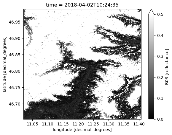
As a first step we will create a RGB data cube from Sentinel-2, including a cloud cover map (CLM). This can be useful to visualize the Sentinel-2 images for some specific date. The spatial resolution set for this cube will be 0.00018 degree, which correspond roughly to the native 10 meter resolution of the Sentinel-2 visible bands (B02: blue, B03: green, B04: red)
cube_config_s2rgb = CubeConfig(
    dataset_name='S2L2A',
    band_names=['B02', 'B03', 'B04', 'CLM'],
    bbox=bbox.tolist(),
    spatial_res=0.00018,
    time_range=[start_date.strftime("%Y-%m-%d"), end_date.strftime("%Y-%m-%d")]
)
/home/conda/master-asi-conae/315434deb1b1e05eacacc41e1b0529b1837100f46402a32041d77ba54ae6c5f3-20230213-125825-013239-74-edc-2022.10-14/lib/python3.9/site-packages/xcube_sh/config.py:248: FutureWarning: Units 'M', 'Y' and 'y' do not represent unambiguous timedelta values and will be removed in a future version.
  time_tolerance = pd.to_timedelta(time_tolerance)
Loading the data into the cube
cube_s2rgb = open_cube(cube_config_s2rgb)
cube_s2rgb
<xarray.Dataset>
Dimensions:    (time: 58, lat: 1864, lon: 2146, bnds: 2)
Coordinates:
  * lat        (lat) float64 46.99 46.99 46.99 46.99 ... 46.65 46.65 46.65 46.65
  * lon        (lon) float64 11.02 11.02 11.02 11.02 ... 11.41 11.41 11.41 11.41
  * time       (time) datetime64[ns] 2018-02-01T10:22:37 ... 2018-06-28T10:13:58
    time_bnds  (time, bnds) datetime64[ns] dask.array<chunksize=(58, 2), meta=np.ndarray>
Dimensions without coordinates: bnds
Data variables:
    B02        (time, lat, lon) float32 dask.array<chunksize=(1, 932, 1073), meta=np.ndarray>
    B03        (time, lat, lon) float32 dask.array<chunksize=(1, 932, 1073), meta=np.ndarray>
    B04        (time, lat, lon) float32 dask.array<chunksize=(1, 932, 1073), meta=np.ndarray>
    CLM        (time, lat, lon) float32 dask.array<chunksize=(1, 932, 1073), meta=np.ndarray>
Attributes:
    Conventions:             CF-1.7
    title:                   S2L2A Data Cube Subset
    history:                 [{'program': 'xcube_sh.chunkstore.SentinelHubChu...
    date_created:            2023-02-21T09:43:08.149994
    time_coverage_start:     2018-02-01T10:22:37+00:00
    time_coverage_end:       2018-06-28T10:13:58+00:00
    time_coverage_duration:  P146DT23H51M21S
    geospatial_lon_min:      11.020833333333357
    geospatial_lat_min:      46.653599378797765
    geospatial_lon_max:      11.407113333333356
    geospatial_lat_max:      46.98911937879777
processing_level: L2AShow the date list of the data in the cube
cube_s2rgb.time
<xarray.DataArray 'time' (time: 58)>
array(['2018-02-01T10:22:37.000000000', '2018-02-03T10:12:37.000000000',
       '2018-02-06T10:22:06.000000000', '2018-02-08T10:11:53.000000000',
       '2018-02-11T10:25:59.000000000', '2018-02-13T10:15:59.000000000',
       '2018-02-16T10:26:01.000000000', '2018-02-18T10:13:13.000000000',
       '2018-02-21T10:20:33.000000000', '2018-02-23T10:15:08.000000000',
       '2018-02-26T10:20:50.000000000', '2018-02-28T10:10:21.000000000',
       '2018-03-03T10:27:07.000000000', '2018-03-05T10:13:15.000000000',
       '2018-03-08T10:22:41.000000000', '2018-03-10T10:10:20.000000000',
       '2018-03-13T10:25:40.000000000', '2018-03-15T10:10:38.000000000',
       '2018-03-20T10:10:21.000000000', '2018-03-23T10:20:21.000000000',
       '2018-03-25T10:15:11.000000000', '2018-03-28T10:23:58.000000000',
       '2018-03-30T10:16:20.000000000', '2018-04-02T10:24:35.000000000',
       '2018-04-04T10:10:21.000000000', '2018-04-07T10:20:20.000000000',
       '2018-04-09T10:13:43.000000000', '2018-04-12T10:20:24.000000000',
       '2018-04-14T10:15:36.000000000', '2018-04-17T10:20:21.000000000',
       '2018-04-19T10:14:57.000000000', '2018-04-22T10:21:15.000000000',
       '2018-04-24T10:15:26.000000000', '2018-04-27T10:20:22.000000000',
       '2018-04-29T10:12:58.000000000', '2018-05-02T10:24:34.000000000',
       '2018-05-04T10:10:23.000000000', '2018-05-07T10:26:48.000000000',
       '2018-05-09T10:16:21.000000000', '2018-05-12T10:21:48.000000000',
       '2018-05-14T10:10:52.000000000', '2018-05-17T10:22:09.000000000',
       '2018-05-19T10:12:07.000000000', '2018-05-22T10:20:25.000000000',
       '2018-05-24T10:10:22.000000000', '2018-05-29T10:12:25.000000000',
       '2018-06-01T10:20:24.000000000', '2018-06-03T10:13:29.000000000',
       '2018-06-06T10:25:12.000000000', '2018-06-08T10:17:26.000000000',
       '2018-06-11T10:26:34.000000000', '2018-06-13T10:14:24.000000000',
       '2018-06-16T10:20:21.000000000', '2018-06-18T10:17:33.000000000',
       '2018-06-21T10:23:16.000000000', '2018-06-23T10:11:39.000000000',
       '2018-06-26T10:26:26.000000000', '2018-06-28T10:13:58.000000000'],
      dtype='datetime64[ns]')
Coordinates:
* time (time) datetime64[ns] 2018-02-01T10:22:37 ... 2018-06-28T10:13:58
Attributes:
standard_name: time
bounds: time_bndsShow a band image for one date
cube_s2rgb.B03.sel(time='2018-04-02T10:24:35.000000000')
<xarray.DataArray 'B03' (lat: 1864, lon: 2146)>
dask.array<getitem, shape=(1864, 2146), dtype=float32, chunksize=(932, 1073), chunktype=numpy.ndarray>
Coordinates:
  * lat      (lat) float64 46.99 46.99 46.99 46.99 ... 46.65 46.65 46.65 46.65
  * lon      (lon) float64 11.02 11.02 11.02 11.02 ... 11.41 11.41 11.41 11.41
    time     datetime64[ns] 2018-04-02T10:24:35
Attributes:
    sample_type:   FLOAT32
    units:         reflectance
    wavelength:    559.4
    wavelength_a:  559.8
    wavelength_b:  559
    bandwidth:     36.0
    bandwidth_a:   36
    bandwidth_b:   36
resolution: 10cube_s2rgb.B03.sel(time='2018-04-02T10:24:35.000000000').plot.imshow(vmin=0, vmax=0.5, cmap='gray')
<matplotlib.image.AxesImage at 0x7fd4866e9e80>
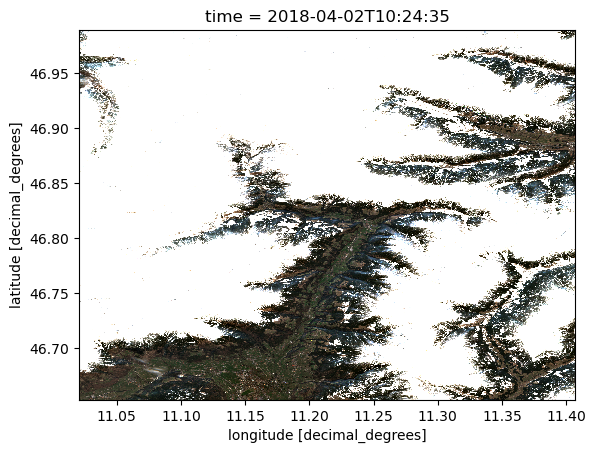
Show the RGB image for the same date
cube_s2rgb[['B04', 'B03', 'B02']].sel(time='2018-04-02T10:24:35.000000000').to_array().plot.imshow(vmin=0, vmax=0.3)
<matplotlib.image.AxesImage at 0x7fd486ba3cd0>
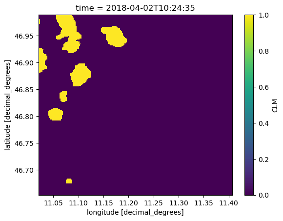
Show the cloud mask for the same date
cube_s2rgb.CLM.sel(time='2018-04-02T10:24:35.000000000').plot.imshow()
<matplotlib.image.AxesImage at 0x7fd486b389a0>
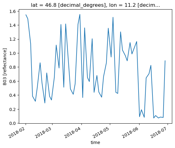
Show a pixel time series for one band
cube_s2rgb.B03.sel(lat=46.8, lon=11.2, method='nearest').plot()
[<matplotlib.lines.Line2D at 0x7fd486a67c40>]
Create the snowmap data cube#
After cloud masking, snow map can be obtained by thresholding the Normalized Difference Snow Index (NDSI) which is computed as:
We will therefore create a Sentinel-2 data cube with bands B03 (green), B11 (SWIR) and the cloud mask (CLM). To speed up the computation of the SCA we will set the resolution equal to 0.0018 degrees, which correspond roughly to 100 m. This resolution is generally enough to get reliable estimate of snow cover area over a catchment.
cube_config_s2snowmap = CubeConfig(
    dataset_name='S2L2A',
    band_names=['B03', 'B11', 'CLM'],
    bbox=bbox.tolist(),
    spatial_res=0.0018,
    time_range=[start_date.strftime("%Y-%m-%d"), end_date.strftime("%Y-%m-%d")],
    downsampling='BILINEAR'
)
/home/conda/master-asi-conae/315434deb1b1e05eacacc41e1b0529b1837100f46402a32041d77ba54ae6c5f3-20230213-125825-013239-74-edc-2022.10-14/lib/python3.9/site-packages/xcube_sh/config.py:248: FutureWarning: Units 'M', 'Y' and 'y' do not represent unambiguous timedelta values and will be removed in a future version.
  time_tolerance = pd.to_timedelta(time_tolerance)
cube_s2snowmap = open_cube(cube_config_s2snowmap)
cube_s2snowmap
<xarray.Dataset>
Dimensions:    (time: 58, lat: 167, lon: 192, bnds: 2)
Coordinates:
  * lat        (lat) float64 46.95 46.95 46.95 46.95 ... 46.66 46.66 46.66 46.65
  * lon        (lon) float64 11.02 11.02 11.03 11.03 ... 11.36 11.36 11.36 11.37
  * time       (time) datetime64[ns] 2018-02-01T10:22:37 ... 2018-06-28T10:13:58
    time_bnds  (time, bnds) datetime64[ns] dask.array<chunksize=(58, 2), meta=np.ndarray>
Dimensions without coordinates: bnds
Data variables:
    B03        (time, lat, lon) float32 dask.array<chunksize=(1, 167, 192), meta=np.ndarray>
    B11        (time, lat, lon) float32 dask.array<chunksize=(1, 167, 192), meta=np.ndarray>
    CLM        (time, lat, lon) float32 dask.array<chunksize=(1, 167, 192), meta=np.ndarray>
Attributes:
    Conventions:             CF-1.7
    title:                   S2L2A Data Cube Subset
    history:                 [{'program': 'xcube_sh.chunkstore.SentinelHubChu...
    date_created:            2023-02-17T09:42:47.174581
    time_coverage_start:     2018-02-01T10:22:37+00:00
    time_coverage_end:       2018-06-28T10:13:58+00:00
    time_coverage_duration:  P146DT23H51M21S
    geospatial_lon_min:      11.020833333333357
    geospatial_lat_min:      46.653599378797765
    geospatial_lon_max:      11.366433333333356
    geospatial_lat_max:      46.95419937879777
processing_level: L2ACompute the NDSI and add it to the cube
ndsi=(cube_s2snowmap.B03 - cube_s2snowmap.B11) / (cube_s2snowmap.B03 + cube_s2snowmap.B11)

ndsi.attrs['long_name']='Normalized Difference Snow Index'
ndsi.attrs['units']='unitless'

cube_s2snowmap['NDSI']=ndsi
Visualize an NDSI image for a specific date
cube_s2snowmap.NDSI.sel(time='2018-04-02T10:24:35.000000000').plot.imshow(vmin=-1, vmax=1, cmap='gray')
<matplotlib.image.AxesImage at 0x7f4ba899e730>
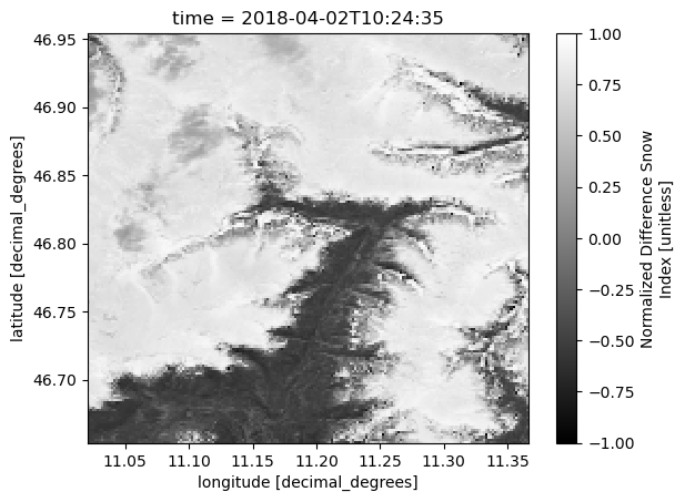
Create the snow cover maps by setting a threshold equal to 0.4 on the NDSI
cube_s2snowmap['snowmap'] = cube_s2snowmap.NDSI > 0.4
cube_s2snowmap
<xarray.Dataset>
Dimensions:    (time: 58, lat: 167, lon: 192, bnds: 2)
Coordinates:
  * lat        (lat) float64 46.95 46.95 46.95 46.95 ... 46.66 46.66 46.66 46.65
  * lon        (lon) float64 11.02 11.02 11.03 11.03 ... 11.36 11.36 11.36 11.37
  * time       (time) datetime64[ns] 2018-02-01T10:22:37 ... 2018-06-28T10:13:58
    time_bnds  (time, bnds) datetime64[ns] dask.array<chunksize=(58, 2), meta=np.ndarray>
Dimensions without coordinates: bnds
Data variables:
    B03        (time, lat, lon) float32 dask.array<chunksize=(1, 167, 192), meta=np.ndarray>
    B11        (time, lat, lon) float32 dask.array<chunksize=(1, 167, 192), meta=np.ndarray>
    CLM        (time, lat, lon) float32 dask.array<chunksize=(1, 167, 192), meta=np.ndarray>
    NDSI       (time, lat, lon) float32 dask.array<chunksize=(1, 167, 192), meta=np.ndarray>
    snowmap    (time, lat, lon) bool dask.array<chunksize=(1, 167, 192), meta=np.ndarray>
Attributes:
    Conventions:             CF-1.7
    title:                   S2L2A Data Cube Subset
    history:                 [{'program': 'xcube_sh.chunkstore.SentinelHubChu...
    date_created:            2023-02-17T09:42:47.174581
    time_coverage_start:     2018-02-01T10:22:37+00:00
    time_coverage_end:       2018-06-28T10:13:58+00:00
    time_coverage_duration:  P146DT23H51M21S
    geospatial_lon_min:      11.020833333333357
    geospatial_lat_min:      46.653599378797765
    geospatial_lon_max:      11.366433333333356
    geospatial_lat_max:      46.95419937879777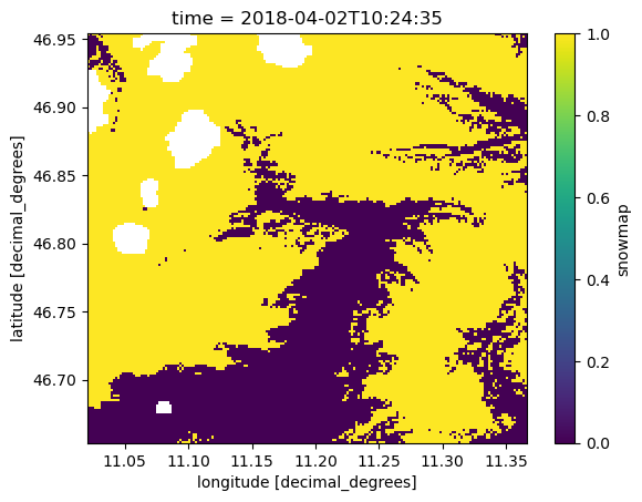
processing_level: L2AAdd the cloud mask
cube_s2snowmap['snowmap'] = cube_s2snowmap.snowmap.where(cube_s2snowmap.CLM==0)
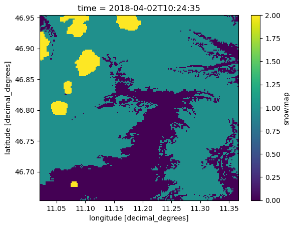
Show a snow map (no snow = 0, snow = 1, cloud = NaN)
cube_s2snowmap.snowmap.sel(time='2018-04-02T10:24:35.000000000').plot.imshow()
<matplotlib.image.AxesImage at 0x7f4ba87cd970>
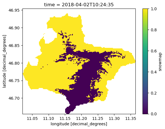
Catchment SCA time series#
Mask with the catchment outline
cube_s2snowmap_masked = mask_dataset_by_geometry(cube_s2snowmap, catchment_outline.iloc[0].geometry)
cube_s2snowmap_masked.snowmap.sel(time='2018-04-02T10:24:35.000000000').plot.imshow()
<matplotlib.image.AxesImage at 0x7f4ba86d4b50>
Compute the cloud percent in the catchment for each Sentinel-2 image
n_cloud = cube_s2snowmap_masked.CLM.sum(dim=['lat', 'lon'])
n_cloud_valid = cube_s2snowmap_masked.CLM.count(dim=['lat', 'lon'])

cube_s2snowmap_masked['cloud_percent'] = n_cloud / n_cloud_valid * 100
cube_s2snowmap_masked
<xarray.Dataset>
Dimensions:        (lat: 166, lon: 191, time: 58, bnds: 2)
Coordinates:
  * lat            (lat) float64 46.95 46.95 46.95 46.95 ... 46.66 46.66 46.66
  * lon            (lon) float64 11.02 11.02 11.03 11.03 ... 11.36 11.36 11.36
  * time           (time) datetime64[ns] 2018-02-01T10:22:37 ... 2018-06-28T1...
    time_bnds      (time, bnds) datetime64[ns] dask.array<chunksize=(58, 2), meta=np.ndarray>
Dimensions without coordinates: bnds
Data variables:
    B03            (time, lat, lon) float32 dask.array<chunksize=(1, 166, 191), meta=np.ndarray>
    B11            (time, lat, lon) float32 dask.array<chunksize=(1, 166, 191), meta=np.ndarray>
    CLM            (time, lat, lon) float32 dask.array<chunksize=(1, 166, 191), meta=np.ndarray>
    NDSI           (time, lat, lon) float32 dask.array<chunksize=(1, 166, 191), meta=np.ndarray>
    snowmap        (time, lat, lon) float64 dask.array<chunksize=(1, 166, 191), meta=np.ndarray>
    cloud_percent  (time) float64 dask.array<chunksize=(1,), meta=np.ndarray>
Attributes: (12/17)
    Conventions:                CF-1.7
    title:                      S2L2A Data Cube Subset
    history:                    [{'program': 'xcube_sh.chunkstore.SentinelHub...
    date_created:               2023-02-17T09:42:47.174581
    time_coverage_start:        2018-02-01T10:22:37+00:00
    time_coverage_end:          2018-06-28T10:13:58+00:00
    ...                         ...
    processing_level:           L2A
    geospatial_lon_units:       degrees_east
    geospatial_lon_resolution:  0.0018000000000000028
    geospatial_lat_units:       degrees_north
    geospatial_lat_resolution:  0.0017999999999999822
date_modified: 2023-02-17T09:43:16.744018In order to get an accurate snow cover area estimation we want to keep only the Sentinel-2 images with a cloud percent in the catchment lower than 20%
cube_s2snowmap_masked = cube_s2snowmap_masked.sel(time=cube_s2snowmap_masked.cloud_percent < 20)
For the remaining image we can then estimate the snow cover area
n_snow = cube_s2snowmap_masked.snowmap.sum(dim=['lat', 'lon'])
n_snow_valid = cube_s2snowmap_masked.snowmap.count(dim=['lat', 'lon'])

cube_s2snowmap_masked['snow_percent'] = n_snow / n_snow_valid * 100
The snow and cloud percentage value can be represented in a pandas DataFrame and saved as csv
sca_ts = cube_s2snowmap_masked[['cloud_percent', 'snow_percent']].to_dataframe()
sca_ts
| cloud_percent | snow_percent | |
|---|---|---|
| time | ||
| 2018-02-08 10:11:53 | 14.107938 | 79.586701 |
| 2018-02-11 10:25:59 | 4.827089 | 74.475260 |
| 2018-02-13 10:15:59 | 18.384857 | 68.060348 |
| 2018-02-21 10:20:33 | 0.000000 | 71.934766 |
| 2018-02-28 10:10:21 | 12.765261 | 68.030633 |
| 2018-03-08 10:22:41 | 10.734870 | 85.508841 |
| 2018-03-20 10:10:21 | 11.095101 | 78.134669 |
| 2018-03-23 10:20:21 | 14.219282 | 69.458655 |
| 2018-03-25 10:15:11 | 4.466859 | 69.813520 |
| 2018-04-02 10:24:35 | 4.460309 | 68.725578 |
| 2018-04-07 10:20:20 | 0.700812 | 66.367654 |
| 2018-04-14 10:15:36 | 10.178150 | 72.582762 |
| 2018-04-19 10:14:57 | 0.000000 | 58.560388 |
| 2018-04-22 10:21:15 | 0.000000 | 54.872937 |
| 2018-04-24 10:15:26 | 18.273513 | 49.479083 |
| 2018-06-16 10:20:21 | 0.137543 | 6.388142 |
| 2018-06-23 10:11:39 | 3.163479 | 3.645587 |
sca_ts['snow_percent'].to_csv('s2_sca_ts_cloudfree.csv')
sca_ts['snow_percent'].plot(marker='o')
<AxesSubplot: xlabel='time'>
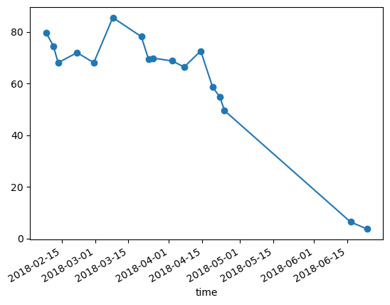
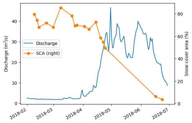
Compare the evolution of SCA to runoff#
In alpine catchment snow represent a major contribution to the runoff during the melting season. As a qualitative analysis we will plot the runoff time series for the selected catchment toghether with the SCA time series we derived from Sentinel-2. As soon as the SCA decreases due to melting, the snow melt contribution implies an increase of the runoff.
Load the runoff time series stored in the csv file:
dsc = pd.read_csv('ADO_DSC_ITH1_0025.csv', sep=',', index_col='Time', parse_dates=True)
dsc
| discharge_m3_s | |
|---|---|
| Time | |
| 1994-01-01 01:00:00 | 4.03 |
| 1994-01-02 01:00:00 | 3.84 |
| 1994-01-03 01:00:00 | 3.74 |
| 1994-01-04 01:00:00 | 3.89 |
| 1994-01-05 01:00:00 | 3.80 |
| ... | ... |
| 2021-07-17 02:00:00 | NaN |
| 2021-07-18 02:00:00 | NaN |
| 2021-07-19 02:00:00 | NaN |
| 2021-07-20 02:00:00 | NaN |
| 2021-07-21 02:00:00 | NaN |
10064 rows × 1 columns
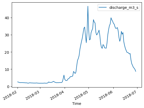
Select the runoff time series accordingly with the time period we used to estimate the Sentinel-2 SCA
dsc = dsc.loc[start_date:end_date]
dsc.plot()
<AxesSubplot: xlabel='Time'>
Plot the runoff (left axes, blue line) toghether with the Sentinel-2 SCA (right axes, orange line)
ax1 = dsc.discharge_m3_s.plot(label='Discharge', xlabel='', ylabel='Discharge (m$^3$/s)')
ax2 = sca_ts.snow_percent.plot(marker='o', secondary_y=True, label='SCA', xlabel='', ylabel='Snow cover area (%)')

ax1.legend(loc='center left', bbox_to_anchor=(0, 0.6))
ax2.legend(loc='center left', bbox_to_anchor=(0, 0.5))

plt.show()
cube_s2snowmap['snowmap'] = cube_s2snowmap.snowmap.where(cube_s2snowmap.CLM==0, 2)
cube_s2snowmap.snowmap.sel(time='2018-04-02T10:24:35.000000000').plot.imshow()
<matplotlib.image.AxesImage at 0x7f3fb8709a00>
cube_s2snowmap_masked = mask_dataset_by_geometry(cube_s2snowmap, catchment_outline.iloc[0].geometry, save_geometry_mask=True)
cube_s2snowmap_masked
<xarray.Dataset>
Dimensions:        (lat: 166, lon: 191, time: 58, bnds: 2)
Coordinates:
  * lat            (lat) float64 46.95 46.95 46.95 46.95 ... 46.66 46.66 46.66
  * lon            (lon) float64 11.02 11.02 11.03 11.03 ... 11.36 11.36 11.36
  * time           (time) datetime64[ns] 2018-02-01T10:22:37 ... 2018-06-28T1...
    time_bnds      (time, bnds) datetime64[ns] dask.array<chunksize=(58, 2), meta=np.ndarray>
Dimensions without coordinates: bnds
Data variables:
    B03            (time, lat, lon) float32 dask.array<chunksize=(1, 166, 191), meta=np.ndarray>
    B11            (time, lat, lon) float32 dask.array<chunksize=(1, 166, 191), meta=np.ndarray>
    CLM            (time, lat, lon) float32 dask.array<chunksize=(1, 166, 191), meta=np.ndarray>
    NDSI           (time, lat, lon) float32 dask.array<chunksize=(1, 166, 191), meta=np.ndarray>
    snowmap        (time, lat, lon) float64 dask.array<chunksize=(1, 166, 191), meta=np.ndarray>
    geometry_mask  (lat, lon) bool dask.array<chunksize=(166, 191), meta=np.ndarray>
Attributes: (12/17)
    Conventions:                CF-1.7
    title:                      S2L2A Data Cube Subset
    history:                    [{'program': 'xcube_sh.chunkstore.SentinelHub...
    date_created:               2023-02-17T09:40:08.516335
    time_coverage_start:        2018-02-01T10:22:37+00:00
    time_coverage_end:          2018-06-28T10:13:58+00:00
    ...                         ...
    processing_level:           L2A
    geospatial_lon_units:       degrees_east
    geospatial_lon_resolution:  0.0018000000000000028
    geospatial_lat_units:       degrees_north
    geospatial_lat_resolution:  0.0017999999999999822
date_modified: 2023-02-17T09:40:51.289454cube_s2snowmap_masked['CLM'] = cube_s2snowmap_masked.CLM == 1
cube_s2snowmap_masked
<xarray.Dataset>
Dimensions:        (lat: 166, lon: 191, time: 58, bnds: 2)
Coordinates:
  * lat            (lat) float64 46.95 46.95 46.95 46.95 ... 46.66 46.66 46.66
  * lon            (lon) float64 11.02 11.02 11.03 11.03 ... 11.36 11.36 11.36
  * time           (time) datetime64[ns] 2018-02-01T10:22:37 ... 2018-06-28T1...
    time_bnds      (time, bnds) datetime64[ns] dask.array<chunksize=(58, 2), meta=np.ndarray>
Dimensions without coordinates: bnds
Data variables:
    B03            (time, lat, lon) float32 dask.array<chunksize=(1, 166, 191), meta=np.ndarray>
    B11            (time, lat, lon) float32 dask.array<chunksize=(1, 166, 191), meta=np.ndarray>
    CLM            (time, lat, lon) bool dask.array<chunksize=(1, 166, 191), meta=np.ndarray>
    NDSI           (time, lat, lon) float32 dask.array<chunksize=(1, 166, 191), meta=np.ndarray>
    snowmap        (time, lat, lon) float64 dask.array<chunksize=(1, 166, 191), meta=np.ndarray>
    geometry_mask  (lat, lon) bool dask.array<chunksize=(166, 191), meta=np.ndarray>
Attributes: (12/17)
    Conventions:                CF-1.7
    title:                      S2L2A Data Cube Subset
    history:                    [{'program': 'xcube_sh.chunkstore.SentinelHub...
    date_created:               2023-02-17T09:40:08.516335
    time_coverage_start:        2018-02-01T10:22:37+00:00
    time_coverage_end:          2018-06-28T10:13:58+00:00
    ...                         ...
    processing_level:           L2A
    geospatial_lon_units:       degrees_east
    geospatial_lon_resolution:  0.0018000000000000028
    geospatial_lat_units:       degrees_north
    geospatial_lat_resolution:  0.0017999999999999822
date_modified: 2023-02-17T09:40:51.289454n_cloud = cube_s2snowmap_masked.CLM.sum(dim=['lat', 'lon'])
n_valid = cube_s2snowmap_masked.geometry_mask.sum(dim=['lat', 'lon'])
cube_s2snowmap_masked['cloud_percent'] = n_cloud / n_valid * 100
cube_s2snowmap_masked
<xarray.Dataset>
Dimensions:        (lat: 166, lon: 191, time: 58, bnds: 2)
Coordinates:
  * lat            (lat) float64 46.95 46.95 46.95 46.95 ... 46.66 46.66 46.66
  * lon            (lon) float64 11.02 11.02 11.03 11.03 ... 11.36 11.36 11.36
  * time           (time) datetime64[ns] 2018-02-01T10:22:37 ... 2018-06-28T1...
    time_bnds      (time, bnds) datetime64[ns] dask.array<chunksize=(58, 2), meta=np.ndarray>
Dimensions without coordinates: bnds
Data variables:
    B03            (time, lat, lon) float32 dask.array<chunksize=(1, 166, 191), meta=np.ndarray>
    B11            (time, lat, lon) float32 dask.array<chunksize=(1, 166, 191), meta=np.ndarray>
    CLM            (time, lat, lon) bool dask.array<chunksize=(1, 166, 191), meta=np.ndarray>
    NDSI           (time, lat, lon) float32 dask.array<chunksize=(1, 166, 191), meta=np.ndarray>
    snowmap        (time, lat, lon) float64 dask.array<chunksize=(1, 166, 191), meta=np.ndarray>
    geometry_mask  (lat, lon) bool dask.array<chunksize=(166, 191), meta=np.ndarray>
    cloud_percent  (time) float64 dask.array<chunksize=(1,), meta=np.ndarray>
Attributes: (12/17)
    Conventions:                CF-1.7
    title:                      S2L2A Data Cube Subset
    history:                    [{'program': 'xcube_sh.chunkstore.SentinelHub...
    date_created:               2023-02-17T09:40:08.516335
    time_coverage_start:        2018-02-01T10:22:37+00:00
    time_coverage_end:          2018-06-28T10:13:58+00:00
    ...                         ...
    processing_level:           L2A
    geospatial_lon_units:       degrees_east
    geospatial_lon_resolution:  0.0018000000000000028
    geospatial_lat_units:       degrees_north
    geospatial_lat_resolution:  0.0017999999999999822
date_modified: 2023-02-17T09:40:51.289454cube_s2snowmap_masked = cube_s2snowmap_masked.sel(time=cube_s2snowmap_masked.cloud_percent < 20)
cube_s2snowmap_masked
<xarray.Dataset>
Dimensions:        (lat: 166, lon: 191, time: 17, bnds: 2)
Coordinates:
  * lat            (lat) float64 46.95 46.95 46.95 46.95 ... 46.66 46.66 46.66
  * lon            (lon) float64 11.02 11.02 11.03 11.03 ... 11.36 11.36 11.36
  * time           (time) datetime64[ns] 2018-02-08T10:11:53 ... 2018-06-23T1...
    time_bnds      (time, bnds) datetime64[ns] dask.array<chunksize=(17, 2), meta=np.ndarray>
Dimensions without coordinates: bnds
Data variables:
    B03            (time, lat, lon) float32 dask.array<chunksize=(1, 166, 191), meta=np.ndarray>
    B11            (time, lat, lon) float32 dask.array<chunksize=(1, 166, 191), meta=np.ndarray>
    CLM            (time, lat, lon) bool dask.array<chunksize=(1, 166, 191), meta=np.ndarray>
    NDSI           (time, lat, lon) float32 dask.array<chunksize=(1, 166, 191), meta=np.ndarray>
    snowmap        (time, lat, lon) float64 dask.array<chunksize=(1, 166, 191), meta=np.ndarray>
    geometry_mask  (lat, lon) bool dask.array<chunksize=(166, 191), meta=np.ndarray>
    cloud_percent  (time) float64 dask.array<chunksize=(1,), meta=np.ndarray>
Attributes: (12/17)
    Conventions:                CF-1.7
    title:                      S2L2A Data Cube Subset
    history:                    [{'program': 'xcube_sh.chunkstore.SentinelHub...
    date_created:               2023-02-17T09:40:08.516335
    time_coverage_start:        2018-02-01T10:22:37+00:00
    time_coverage_end:          2018-06-28T10:13:58+00:00
    ...                         ...
    processing_level:           L2A
    geospatial_lon_units:       degrees_east
    geospatial_lon_resolution:  0.0018000000000000028
    geospatial_lat_units:       degrees_north
    geospatial_lat_resolution:  0.0017999999999999822
date_modified: 2023-02-17T09:40:51.289454cube_s2snowmap_masked['snowmap'] = cube_s2snowmap_masked.snowmap == 1
n_snow = cube_s2snowmap_masked.snowmap.sum(dim=['lat', 'lon'])

cube_s2snowmap_masked['snow_percent'] = n_snow / (n_valid - n_cloud) * 100
cube_s2snowmap_masked
<xarray.Dataset>
Dimensions:        (lat: 166, lon: 191, time: 17, bnds: 2)
Coordinates:
  * lat            (lat) float64 46.95 46.95 46.95 46.95 ... 46.66 46.66 46.66
  * lon            (lon) float64 11.02 11.02 11.03 11.03 ... 11.36 11.36 11.36
  * time           (time) datetime64[ns] 2018-02-08T10:11:53 ... 2018-06-23T1...
    time_bnds      (time, bnds) datetime64[ns] dask.array<chunksize=(17, 2), meta=np.ndarray>
Dimensions without coordinates: bnds
Data variables:
    B03            (time, lat, lon) float32 dask.array<chunksize=(1, 166, 191), meta=np.ndarray>
    B11            (time, lat, lon) float32 dask.array<chunksize=(1, 166, 191), meta=np.ndarray>
    CLM            (time, lat, lon) bool dask.array<chunksize=(1, 166, 191), meta=np.ndarray>
    NDSI           (time, lat, lon) float32 dask.array<chunksize=(1, 166, 191), meta=np.ndarray>
    snowmap        (time, lat, lon) bool dask.array<chunksize=(1, 166, 191), meta=np.ndarray>
    geometry_mask  (lat, lon) bool dask.array<chunksize=(166, 191), meta=np.ndarray>
    cloud_percent  (time) float64 dask.array<chunksize=(1,), meta=np.ndarray>
    snow_percent   (time) float64 dask.array<chunksize=(1,), meta=np.ndarray>
Attributes: (12/17)
    Conventions:                CF-1.7
    title:                      S2L2A Data Cube Subset
    history:                    [{'program': 'xcube_sh.chunkstore.SentinelHub...
    date_created:               2023-02-17T09:40:08.516335
    time_coverage_start:        2018-02-01T10:22:37+00:00
    time_coverage_end:          2018-06-28T10:13:58+00:00
    ...                         ...
    processing_level:           L2A
    geospatial_lon_units:       degrees_east
    geospatial_lon_resolution:  0.0018000000000000028
    geospatial_lat_units:       degrees_north
    geospatial_lat_resolution:  0.0017999999999999822
date_modified: 2023-02-17T09:40:51.289454sca_ts = cube_s2snowmap_masked[['cloud_percent', 'snow_percent']].to_dataframe()
sca_ts
| cloud_percent | snow_percent | |
|---|---|---|
| time | ||
| 2018-02-08 10:11:53 | 14.107938 | 79.586701 |
| 2018-02-11 10:25:59 | 4.827089 | 74.475260 |
| 2018-02-13 10:15:59 | 18.384857 | 68.060348 |
| 2018-02-21 10:20:33 | 0.000000 | 71.934766 |
| 2018-02-28 10:10:21 | 12.765261 | 68.030633 |
| 2018-03-08 10:22:41 | 10.734870 | 85.508841 |
| 2018-03-20 10:10:21 | 11.095101 | 78.134669 |
| 2018-03-23 10:20:21 | 14.219282 | 69.458655 |
| 2018-03-25 10:15:11 | 4.466859 | 69.813520 |
| 2018-04-02 10:24:35 | 4.460309 | 68.725578 |
| 2018-04-07 10:20:20 | 0.700812 | 66.367654 |
| 2018-04-14 10:15:36 | 10.178150 | 72.582762 |
| 2018-04-19 10:14:57 | 0.000000 | 58.560388 |
| 2018-04-22 10:21:15 | 0.000000 | 54.872937 |
| 2018-04-24 10:15:26 | 18.273513 | 49.479083 |
| 2018-06-16 10:20:21 | 0.137543 | 6.388142 |
| 2018-06-23 10:11:39 | 3.163479 | 3.645587 |