![]()
3.2 Validation#
In this exercise, we focus on the validation of the results we have produced. In general, the accuracy of a satellite derived product is expressed by comparing it to in-situ measurements. Furthermore, we will compare the resuling snow cover time series to the runoff of the catchment to check the plausibility of the observed relationship.
The steps involved in this analysis:
Generate Datacube time-series of snowmap,
Load in-situ datasets: snow depth station measurements,
Pre-process and filter in-situ datasets to match area of interest,
Perform validation of snow-depth measurements,
Plausibility check with runoff of the catchment
More information on the openEO Python Client: https://open-eo.github.io/openeo-python-client/index.html
Start by creating the folders and data files needed to complete the exercise.
!cp -r $DATA_PATH/32_results/ $HOME/
!cp -r $DATA_PATH/32_data/ $HOME/
!cp -r $DATA_PATH/_32_cubes_utilities.py $HOME/
Libraries#
import json
from datetime import date
import numpy as np
import pandas as pd

import xarray as xr
import rioxarray as rio

import matplotlib.pyplot as plt
import rasterio
from rasterio.plot import show

import geopandas as gpd
import leafmap.foliumap as leafmap

import openeo
from _32_cubes_utilities import ( calculate_sca,
                                 station_temporal_filter,
                                 station_spatial_filter,
                                 binarize_snow,
                                 format_date,
                                 assign_site_snow,
                                 validation_metrics)
/tmp/ipykernel_1286/2944796695.py:4: DeprecationWarning:
Pyarrow will become a required dependency of pandas in the next major release of pandas (pandas 3.0),
(to allow more performant data types, such as the Arrow string type, and better interoperability with other libraries)
but was not found to be installed on your system.
If this would cause problems for you,
please provide us feedback at https://github.com/pandas-dev/pandas/issues/54466

  import pandas as pd
Login#
Connect to the Copernicus Dataspace Ecosystem.
conn = openeo.connect('https://openeo.dataspace.copernicus.eu/')
Login.
conn.authenticate_oidc()
Authenticated using refresh token.
<Connection to 'https://openeo.dataspace.copernicus.eu/openeo/1.2/' with OidcBearerAuth>
Check if the login worked.
conn.describe_account()
Region of Interest#
Load the Val Passiria Catchment, our region of interest. And plot it.
catchment_outline = gpd.read_file('32_data/catchment_outline.geojson')
center = (float(catchment_outline.centroid.y), float(catchment_outline.centroid.x))
m = leafmap.Map(center=center, zoom=10)
m.add_vector('32_data/catchment_outline.geojson', layer_name="catchment")
m
Generate Datacube of Snowmap#
We have prepared the workflow to generate the snow map as a python function calculate_sca(). The calculate_sca() is from _32_cubes_utilities and is used to reproduce the snow map process graph in openEO
bbox = catchment_outline.bounds.iloc[0]
temporal_extent = ["2018-02-01", "2018-06-30"]
snow_map_cloud_free = calculate_sca(conn, bbox, temporal_extent)
snow_map_cloud_free
Load snow-station in-situ data#
Load the in-situ datasets, snow depth station measurements. They have been compiled in the ClirSnow project and are available here: Snow Cover in the European Alps with stations in our area of interest.
We have made the data available for you already. We can load it directly.
# load snow station datasets from zenodo:: https://zenodo.org/record/5109574
station_df = pd.read_csv("32_data/data_daily_IT_BZ.csv")
station_df = station_df.assign(Date=station_df.apply(format_date, axis=1))
# the format_date function, from _32_cubes_utilities was used to stringify each Datetime object in the dataframe
# station_df.head()
# load additional metadata for acessing the station geometries
station_df_meta = pd.read_csv("32_data/meta_all.csv")
station_df_meta.head()
| Provider | Name | Longitude | Latitude | Elevation | HN_year_start | HN_year_end | HS_year_start | HS_year_end | |
|---|---|---|---|---|---|---|---|---|---|
| 0 | AT_HZB | Absdorf | 15.976667 | 48.401667 | 182.0 | 1970.0 | 2016.0 | 1970.0 | 2016.0 |
| 1 | AT_HZB | Ach_Burghausen | 12.846389 | 48.148889 | 473.0 | 1990.0 | 2016.0 | 1990.0 | 2016.0 |
| 2 | AT_HZB | Admont | 14.457222 | 47.567778 | 700.0 | 1970.0 | 2016.0 | 1970.0 | 2016.0 |
| 3 | AT_HZB | Afritz | 13.795556 | 46.727500 | 715.0 | 1970.0 | 2016.0 | 1970.0 | 2016.0 |
| 4 | AT_HZB | Alberschwende | 9.849167 | 47.458333 | 717.0 | 1982.0 | 2016.0 | 1982.0 | 2016.0 |
Pre-process and filter in-situ snow station measurements#
Filter Temporally#
Filter the in-situ datasets to match the snow-map time series using the function station_temporal_filter() from cubes_utilities.py, which merges the station dataframe with additional metadata needed for the Lat/Long information and convert them to geometries
start_date = "2018-02-01"
end_date = "2018-06-30"

snow_stations = station_temporal_filter(station_daily_df = station_df,
                                        station_meta_df = station_df_meta,
                                        start_date = start_date,
                                        end_date = end_date)
snow_stations.head()
| Provider | Name | Date | HN | HS | HN_after_qc | HS_after_qc | HS_after_gapfill | Longitude | Latitude | Elevation | geometry | |
|---|---|---|---|---|---|---|---|---|---|---|---|---|
| Date | ||||||||||||
| 2018-02-01 | IT_BZ | Diga_di_Neves_Osservatore | 2018-02-01 | 2.0 | 11.0 | 2.0 | NaN | 120.0 | 11.787089 | 46.941417 | 1860.0 | POINT (11.78709 46.94142) |
| 2018-02-01 | IT_BZ | Maia_Alta_Osservatore | 2018-02-01 | 0.0 | 0.0 | 0.0 | 0.0 | 0.0 | 11.183234 | 46.657820 | 334.0 | POINT (11.18323 46.65782) |
| 2018-02-01 | IT_BZ | Racines_di_Dentro_Osservatore | 2018-02-01 | 1.0 | 57.0 | 1.0 | 57.0 | 57.0 | 11.317197 | 46.866026 | 1260.0 | POINT (11.31720 46.86603) |
| 2018-02-01 | IT_BZ | Valles_osservatore | 2018-02-01 | 0.0 | 43.0 | 0.0 | 43.0 | 43.0 | 11.630696 | 46.838655 | 1352.0 | POINT (11.63070 46.83866) |
| 2018-02-01 | IT_BZ | Terento_Osservatore | 2018-02-01 | 0.0 | 9.0 | 0.0 | 9.0 | 9.0 | 11.793769 | 46.832116 | 1240.0 | POINT (11.79377 46.83212) |
Filter Spatially#
Filter the in-situ datasets into the catchment area of interest using station_spatial_filter() from cubes_utilities.py.
catchment_stations = station_spatial_filter(snow_stations, catchment_outline)
catchment_stations.head()
| Provider | Name | HN | HS | HN_after_qc | HS_after_qc | HS_after_gapfill | Longitude | Latitude | Elevation | geometry | |
|---|---|---|---|---|---|---|---|---|---|---|---|
| Date | |||||||||||
| 2018-02-01 | IT_BZ | S_Martino_in_Passiria_Osservatore | 0.0 | 0.0 | 0.0 | 0.0 | 0.0 | 11.227909 | 46.782682 | 588.0 | POINT (11.22791 46.78268) |
| 2018-02-01 | IT_BZ | Rifiano_Beobachter | 0.0 | 0.0 | 0.0 | 0.0 | 0.0 | 11.183607 | 46.705034 | 500.0 | POINT (11.18361 46.70503) |
| 2018-02-01 | IT_BZ | Plata_Osservatore | 2.0 | 55.0 | 2.0 | 55.0 | 55.0 | 11.176968 | 46.822847 | 1130.0 | POINT (11.17697 46.82285) |
| 2018-02-01 | IT_BZ | S_Leonardo_in_Passiria_Osservatore | 0.0 | NaN | 0.0 | NaN | NaN | 11.247126 | 46.809062 | 644.0 | POINT (11.24713 46.80906) |
| 2018-02-01 | IT_BZ | Scena_Osservatore | 0.0 | 0.0 | 0.0 | 0.0 | 0.0 | 11.190831 | 46.689596 | 680.0 | POINT (11.19083 46.68960) |
Plot the filtered stations#
Visualize location of snow stations
print("There are", len(np.unique(catchment_stations.Name)), "unique stations within our catchment area of interest")
There are 5 unique stations within our catchment area of interest
Quick Hint: Remember the number of stations within the catchment for the final quiz exercise
Convert snow depth to snow presence#
The stations are measuring snow depth. We only need the binary information on the presence of snow (yes, no). We use the binarize_snow() function from cubes_utilities.py to assign 0 for now snow and 1 for snow in the snow_presence column.
catchment_stations = catchment_stations.assign(snow_presence=catchment_stations.apply(binarize_snow, axis=1))
catchment_stations.head()
| Provider | Name | HN | HS | HN_after_qc | HS_after_qc | HS_after_gapfill | Longitude | Latitude | Elevation | geometry | snow_presence | |
|---|---|---|---|---|---|---|---|---|---|---|---|---|
| Date | ||||||||||||
| 2018-02-01 | IT_BZ | S_Martino_in_Passiria_Osservatore | 0.0 | 0.0 | 0.0 | 0.0 | 0.0 | 11.227909 | 46.782682 | 588.0 | POINT (11.22791 46.78268) | 0 |
| 2018-02-01 | IT_BZ | Rifiano_Beobachter | 0.0 | 0.0 | 0.0 | 0.0 | 0.0 | 11.183607 | 46.705034 | 500.0 | POINT (11.18361 46.70503) | 0 |
| 2018-02-01 | IT_BZ | Plata_Osservatore | 2.0 | 55.0 | 2.0 | 55.0 | 55.0 | 11.176968 | 46.822847 | 1130.0 | POINT (11.17697 46.82285) | 1 |
| 2018-02-01 | IT_BZ | S_Leonardo_in_Passiria_Osservatore | 0.0 | NaN | 0.0 | NaN | NaN | 11.247126 | 46.809062 | 644.0 | POINT (11.24713 46.80906) | 0 |
| 2018-02-01 | IT_BZ | Scena_Osservatore | 0.0 | 0.0 | 0.0 | 0.0 | 0.0 | 11.190831 | 46.689596 | 680.0 | POINT (11.19083 46.68960) | 0 |
Save the pre-processed snow station measurements#
Save snow stations within catchment as GeoJSON
with open("32_results/catchment_stations.geojson", "w") as file:
    file.write(catchment_stations.to_json())
Extract SCA from the data cube per station#
Prepare snow station data for usage in openEO#
Create a buffer of approximately 80 meters (0.00075 degrees) around snow stations and visualize them.
catchment_stations_gpd = gpd.read_file("32_results/catchment_stations.geojson")
mappy =leafmap.Map(center=center, zoom=16)
mappy.add_vector('32_data/catchment_outline.geojson', layer_name="catchment")
mappy.add_gdf(catchment_stations_gpd, layer_name="catchment_station")

catchment_stations_gpd["geometry"] = catchment_stations_gpd.geometry.buffer(0.00075)
mappy.add_gdf(catchment_stations_gpd, layer_name="catchment_station_buffer")
mappy
Convert the unique geometries to Feature Collection to be used in a openEO process.
catchment_stations_fc = json.loads(
    catchment_stations_gpd.geometry.iloc[:5].to_json()
)
Extract SCA from the data cube per station#
We exgtract the SCA value of our data cube at the buffered station locations. Therefore we use the process aggregate_spatial() with the aggregation method median(). This gives us the most common value in the buffer (snow or snowfree).
snowmap_per_station= snow_map_cloud_free.aggregate_spatial(catchment_stations_fc, reducer="median")
snowmap_per_station
Create a batch job on the cloud platform. And start it.
snowmap_cloudfree_json = snowmap_per_station.save_result(format="JSON")
job = snowmap_cloudfree_json.create_job(title="snow_map")
job.start_and_wait()
0:00:00 Job 'j-240215c46f6e4a899346de93a0f534cc': send 'start'
0:00:14 Job 'j-240215c46f6e4a899346de93a0f534cc': running (progress N/A)
0:00:19 Job 'j-240215c46f6e4a899346de93a0f534cc': running (progress N/A)
0:00:25 Job 'j-240215c46f6e4a899346de93a0f534cc': running (progress N/A)
0:00:34 Job 'j-240215c46f6e4a899346de93a0f534cc': running (progress N/A)
0:00:44 Job 'j-240215c46f6e4a899346de93a0f534cc': running (progress N/A)
0:00:56 Job 'j-240215c46f6e4a899346de93a0f534cc': running (progress N/A)
0:01:11 Job 'j-240215c46f6e4a899346de93a0f534cc': running (progress N/A)
0:01:38 Job 'j-240215c46f6e4a899346de93a0f534cc': running (progress N/A)
0:02:02 Job 'j-240215c46f6e4a899346de93a0f534cc': running (progress N/A)
0:02:34 Job 'j-240215c46f6e4a899346de93a0f534cc': running (progress N/A)
0:03:11 Job 'j-240215c46f6e4a899346de93a0f534cc': running (progress N/A)
0:03:58 Job 'j-240215c46f6e4a899346de93a0f534cc': running (progress N/A)
0:04:57 Job 'j-240215c46f6e4a899346de93a0f534cc': finished (progress N/A)
Check the status of the job. And download once it’s finished.
job.status()
'finished'
if job.status() == "finished":
    results = job.get_results()
    results.download_files("32_results/snowmap/")
Open the snow covered area time series extracted at the stations. We’ll have a look at it in a second.
with open("32_results/snowmap/timeseries.json","r") as file:
    snow_time_series = json.load(file)
Combine station measurements and the extracted SCA from our data cube#
The station measurements are daily and all of the stations are combined in one csv file. The extracted SCA values are in the best case six-daily (Sentinel-2 repeat rate) and also all stations are in one json file. We will need to join the the extracted SCA with the station measurements by station (and time (selecting the corresponding time steps)
Extract snow values from SCA extracted at the station location#
Let’s have a look at the data structure first
dates = [k.split("T")[0] for k in snow_time_series]
snow_val_smartino = [snow_time_series[k][0][0] for k in snow_time_series]
snow_val_rifiano = [snow_time_series[k][1][0] for k in snow_time_series]
snow_val_plata = [snow_time_series[k][2][0] for k in snow_time_series]
snow_val_sleonardo = [snow_time_series[k][3][0] for k in snow_time_series]
snow_val_scena = [snow_time_series[k][4][0] for k in snow_time_series]
Match in-situ measurements to dates in SCA#
Let’s have a look at the in-situ measurement data set.
catchment_stations_gpd.sample(10)
| id | Provider | Name | HN | HS | HN_after_qc | HS_after_qc | HS_after_gapfill | Longitude | Latitude | Elevation | snow_presence | geometry | |
|---|---|---|---|---|---|---|---|---|---|---|---|---|---|
| 198 | 2018-03-12 | IT_BZ | Scena_Osservatore | 0.0 | 0.0 | 0.0 | 0.0 | 0.0 | 11.190831 | 46.689596 | 680.0 | 0 | POLYGON ((11.19158 46.68960, 11.19158 46.68952... |
| 13 | 2018-02-03 | IT_BZ | Scena_Osservatore | 0.0 | 0.0 | 0.0 | 0.0 | 0.0 | 11.190831 | 46.689596 | 680.0 | 0 | POLYGON ((11.19158 46.68960, 11.19158 46.68952... |
| 615 | 2018-06-04 | IT_BZ | Rifiano_Beobachter | 0.0 | 0.0 | 0.0 | 0.0 | 0.0 | 11.183607 | 46.705034 | 500.0 | 0 | POLYGON ((11.18436 46.70503, 11.18435 46.70496... |
| 731 | 2018-06-27 | IT_BZ | S_Leonardo_in_Passiria_Osservatore | 0.0 | NaN | 0.0 | NaN | NaN | 11.247126 | 46.809062 | 644.0 | 0 | POLYGON ((11.24788 46.80906, 11.24787 46.80899... |
| 37 | 2018-02-08 | IT_BZ | S_Martino_in_Passiria_Osservatore | 0.0 | 0.0 | 0.0 | 0.0 | 0.0 | 11.227909 | 46.782682 | 588.0 | 0 | POLYGON ((11.22866 46.78268, 11.22866 46.78261... |
| 441 | 2018-04-30 | IT_BZ | Scena_Osservatore | 0.0 | 0.0 | 0.0 | 0.0 | 0.0 | 11.190831 | 46.689596 | 680.0 | 0 | POLYGON ((11.19158 46.68960, 11.19158 46.68952... |
| 691 | 2018-06-19 | IT_BZ | S_Leonardo_in_Passiria_Osservatore | 0.0 | NaN | 0.0 | NaN | NaN | 11.247126 | 46.809062 | 644.0 | 0 | POLYGON ((11.24788 46.80906, 11.24787 46.80899... |
| 614 | 2018-06-03 | IT_BZ | S_Martino_in_Passiria_Osservatore | 0.0 | 0.0 | 0.0 | 0.0 | 0.0 | 11.227909 | 46.782682 | 588.0 | 0 | POLYGON ((11.22866 46.78268, 11.22866 46.78261... |
| 747 | 2018-06-30 | IT_BZ | Rifiano_Beobachter | 0.0 | 0.0 | 0.0 | 0.0 | 0.0 | 11.183607 | 46.705034 | 500.0 | 0 | POLYGON ((11.18436 46.70503, 11.18435 46.70496... |
| 524 | 2018-05-16 | IT_BZ | S_Martino_in_Passiria_Osservatore | 0.0 | 0.0 | 0.0 | 0.0 | 0.0 | 11.227909 | 46.782682 | 588.0 | 0 | POLYGON ((11.22866 46.78268, 11.22866 46.78261... |
We are going to extract each station and keep only the dates that are available in the SCA results.
catchment_stations_gpd_smartino = catchment_stations_gpd.query("Name == 'S_Martino_in_Passiria_Osservatore'")
catchment_stations_gpd_smartino = catchment_stations_gpd_smartino[
    catchment_stations_gpd_smartino.id.isin(dates)
]

catchment_stations_gpd_rifiano = catchment_stations_gpd.query("Name == 'Rifiano_Beobachter'")
catchment_stations_gpd_rifiano = catchment_stations_gpd_rifiano[
    catchment_stations_gpd_rifiano.id.isin(dates)
]

catchment_stations_gpd_plata = catchment_stations_gpd.query("Name == 'Plata_Osservatore'")
catchment_stations_gpd_plata = catchment_stations_gpd_plata[
    catchment_stations_gpd_plata.id.isin(dates)
]

catchment_stations_gpd_sleonardo = catchment_stations_gpd.query("Name == 'S_Leonardo_in_Passiria_Osservatore'")
catchment_stations_gpd_sleonardo = catchment_stations_gpd_sleonardo[
    catchment_stations_gpd_sleonardo.id.isin(dates)
]

catchment_stations_gpd_scena = catchment_stations_gpd.query("Name == 'Scena_Osservatore'")
catchment_stations_gpd_scena = catchment_stations_gpd_scena[
    catchment_stations_gpd_scena.id.isin(dates)
]
Combine in-situ measurements with SCA results at the stations#
The in situ measurements and the SCA are combined into one data set per station. This will be the basis for the validation.
smartino_snow = assign_site_snow(catchment_stations_gpd_smartino, snow_val_smartino)
rifiano_snow = assign_site_snow(catchment_stations_gpd_rifiano, snow_val_rifiano)
plata_snow = assign_site_snow(catchment_stations_gpd_plata, snow_val_plata)
sleonardo_snow = assign_site_snow(catchment_stations_gpd_sleonardo, snow_val_sleonardo)
scena_snow = assign_site_snow(catchment_stations_gpd_scena, snow_val_scena)
Let’s have a look at the SCA extracted at the station San Martino and it’s in situ measurements.
catchment_stations_gpd_plata.sample(5)
| id | Provider | Name | HN | HS | HN_after_qc | HS_after_qc | HS_after_gapfill | Longitude | Latitude | Elevation | snow_presence | geometry | cube_snow | |
|---|---|---|---|---|---|---|---|---|---|---|---|---|---|---|
| 12 | 2018-02-03 | IT_BZ | Plata_Osservatore | 0.0 | 60.0 | 0.0 | 60.0 | 60.0 | 11.176968 | 46.822847 | 1130.0 | 1 | POLYGON ((11.17772 46.82285, 11.17771 46.82277... | NaN |
| 185 | 2018-03-10 | IT_BZ | Plata_Osservatore | 0.0 | 42.0 | 0.0 | 42.0 | 42.0 | 11.176968 | 46.822847 | 1130.0 | 1 | POLYGON ((11.17772 46.82285, 11.17771 46.82277... | NaN |
| 25 | 2018-02-06 | IT_BZ | Plata_Osservatore | 0.0 | 60.0 | 0.0 | 60.0 | 60.0 | 11.176968 | 46.822847 | 1130.0 | 1 | POLYGON ((11.17772 46.82285, 11.17771 46.82277... | NaN |
| 425 | 2018-04-27 | IT_BZ | Plata_Osservatore | 0.0 | 0.0 | 0.0 | 0.0 | 0.0 | 11.176968 | 46.822847 | 1130.0 | 0 | POLYGON ((11.17772 46.82285, 11.17771 46.82277... | NaN |
| 235 | 2018-03-20 | IT_BZ | Plata_Osservatore | 0.0 | 20.0 | 0.0 | 20.0 | 20.0 | 11.176968 | 46.822847 | 1130.0 | 1 | POLYGON ((11.17772 46.82285, 11.17771 46.82277... | 0.0 |
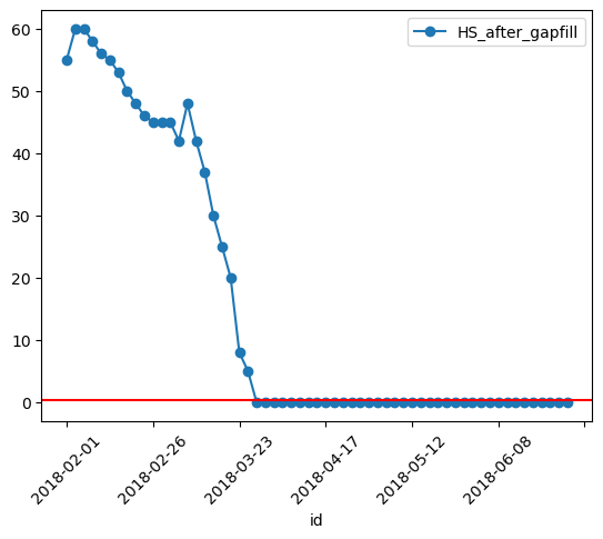
Display snow presence threshold in in-situ data for Plato Osservatore
catchment_stations_gpd_plata.plot(x="id", y="HS_after_gapfill",rot=45,kind="line",marker='o')
plt.axhline(y = 0.4, color = "r", linestyle = "-")
plt.show()
Validate the SCA results with the snow station measurements#
Now that we have combined the SCA results with the snow station measurements we can start the actual validation. A confusion matrix compares the classes of the station data to the classes of the SCA result. The numbers can be used to calculate the accuracy (correctly classified cases / all cases).
no_snow |
snow |
|
|---|---|---|
no_snow |
correct |
error |
snow |
error |
correct |
import seaborn as sns
fig, ((ax1, ax2), (ax3, ax4)) = plt.subplots(2, 2, figsize=(10, 6))

fig.suptitle("Error matrices for snow stations within our selected Catchment")
sns.heatmap(validation_metrics(smartino_snow)[1], annot=True, xticklabels=["No Snow", "Snow"], yticklabels=["No Snow", "Snow"], ax=ax1)
ax1.set_title("San Martino in Passiria Osservatore")
ax1.set(xlabel="Predicted label", ylabel="True label")


sns.heatmap(validation_metrics(rifiano_snow)[1], annot=True, xticklabels=["No Snow", "Snow"], yticklabels=["No Snow", "Snow"], ax=ax2)
ax2.set_title("Rifiano Beobachter")
ax2.set(xlabel="Predicted label", ylabel="True label")


sns.heatmap(validation_metrics(plata_snow)[1], annot=True, xticklabels=["No Snow", "Snow"], yticklabels=["No Snow", "Snow"], ax=ax3)
ax3.set_title("Plata Osservatore")
ax3.set(xlabel="Predicted label", ylabel="True label")


sns.heatmap(validation_metrics(scena_snow)[1], annot=True, xticklabels=["No Snow", "Snow"], yticklabels=["No Snow", "Snow"], ax=ax4)
ax4.set_title("Scena Osservatore")
ax4.set(xlabel="Predicted label", ylabel="True label")

fig.tight_layout()
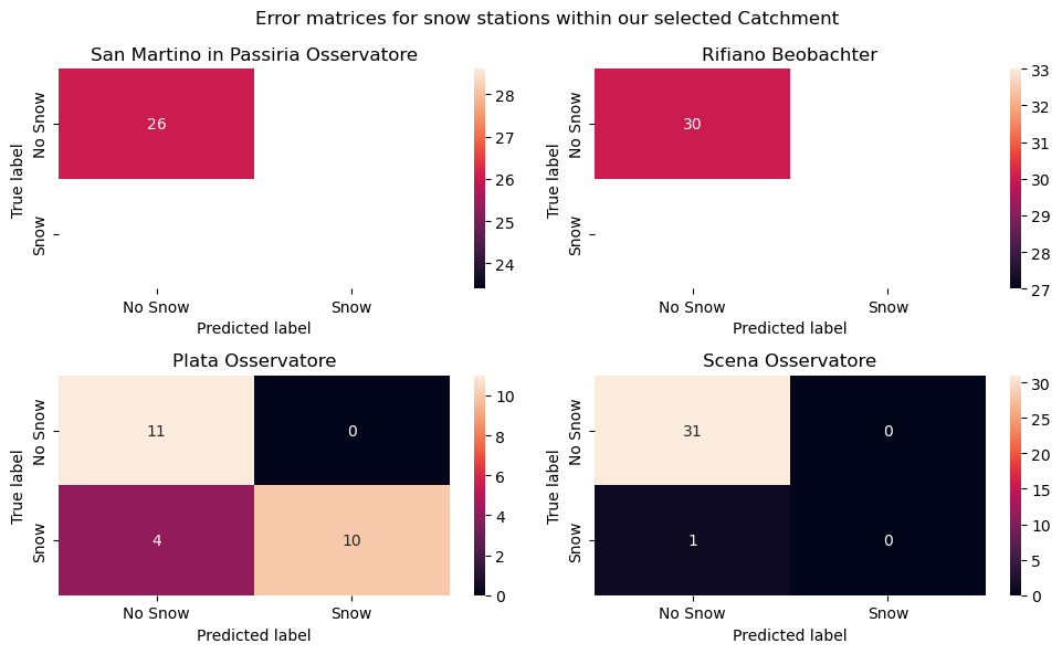
The accuracy of the snow estimate from the satellite image computation for each station is shown below:
On-site snow station |
Accuracy |
|---|---|
San Martino in Passiria Osservatore |
100.00% |
Rifiano Beobachter |
100.00% |
Plata Osservatore |
82.61% |
San Leonardo in Passiria Osservatore |
NaN |
Scena Osservatore |
96.15% |
The fifth and last station San Leonardo in Passiria Osservatore recorded NaNs for snow depths for our selected dates, which could potentially be as a results of malfunctioning on-site equipments. Hence, we are not able to verify for it. But overall, the validation shows a 100% accuracy for stations San Martino in Passiria Osservatore and Rifiano Beobachter, while station Plata Osservatore has a lot more False Positive (4) than the other stations.This shows a good match between estimated snow values from satellite datasets and on-the ground measurements of the presence of snow.
Compare to discharge data#
In addition to computing metrics for validating the data, we also check the plausibility of our results. We compare our results with another measure with a known relationship. In this case, we compare the snow cover area time series with the discharge time-series at the main outlet of the catchment. We suspect that after snow melting starts, with a temporal lag, the runoff will increase. Let’s see if this holds true.
Load the discharge data at Meran, the main outlet of the catchment. We have prepared this data set for you, it’s extracted from Eurac’s Environmental Data Platform Alpine Drought Observatory Discharge Hydrological Datasets).
discharge_ds = pd.read_csv('32_data/ADO_DSC_ITH1_0025.csv',
                           sep=',', index_col='Time', parse_dates=True)
discharge_ds.head()
| discharge_m3_s | |
|---|---|
| Time | |
| 1994-01-01 01:00:00 | 4.03 |
| 1994-01-02 01:00:00 | 3.84 |
| 1994-01-03 01:00:00 | 3.74 |
| 1994-01-04 01:00:00 | 3.89 |
| 1994-01-05 01:00:00 | 3.80 |
Load the SCA time series we have generated in a previous exercise. It’s the time series of the aggregated snow cover area percentage for the whole catchment.
snow_perc_df = pd.read_csv("32_data/filtered_snow_perc.csv",
                          sep=',', index_col='time', parse_dates=True)
Let’s plot the relationship between the snow covered area and the discharge in the catchment.
start_date = date(2018, 2, 1)
end_date = date(2018, 6, 30)
# filter discharge data to start and end dates
discharge_ds = discharge_ds.loc[start_date:end_date]

ax1 = discharge_ds.discharge_m3_s.plot(label='Discharge', xlabel='', ylabel='Discharge (m$^3$/s)')
ax2 = snow_perc_df["perc_snow"].plot(marker='o', secondary_y=True, label='SCA', xlabel='', ylabel='Snow cover area (%)')
ax1.legend(loc='center left', bbox_to_anchor=(0, 0.6))
ax2.legend(loc='center left', bbox_to_anchor=(0, 0.5))
plt.show()
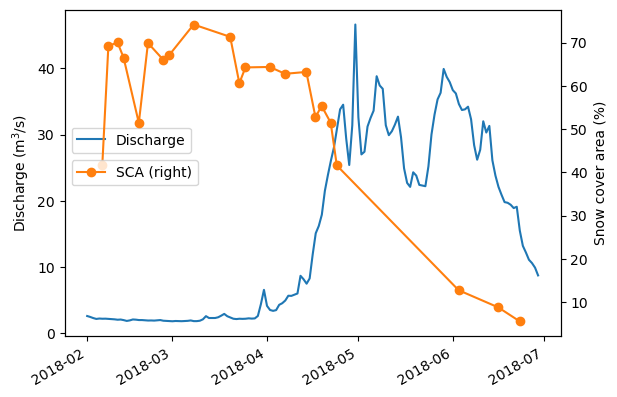
The relationship looks as expected! Once the snow cover decreases the runoff increases!