![]()
3.1 Data Processing#
In this exercise we will build a complete EO workflow on a cloud platform; from data access to obtaining the result. In this example we will analyse snow cover in the Alps.
We are going to follow these steps in our analysis:
Load satellite collections
Specify the spatial, temporal extents and the features we are interested in
Process the satellite data to retrieve snow cover information
aggregate information in data cubes
Visualize and analyse the results
More information on the openEO Python Client: https://open-eo.github.io/openeo-python-client/index.html
Libraries#
%%capture
pip install openeo rioxarray geopandas leafmap h5netcdf netcdf4
# platform libraries
import openeo

# utility libraries
from datetime import date
import numpy as np
import xarray as xr
import rioxarray
import json
import pandas as pd
import matplotlib.pyplot as plt
import geopandas as gpd
import leafmap.foliumap as leafmap
Login#
Connect to the copernicus dataspace ecosystem.
conn = openeo.connect('https://openeo.cloud/')
And login
conn.authenticate_oidc()
Authenticated using refresh token.
<Connection to 'https://openeocloud.vito.be/openeo/1.0.0/' with OidcBearerAuth>
Check if the login worked.
conn.describe_account()
{'default_plan': 'generic',
 'info': {'oidc_userinfo': {'eduperson_assurance': ['https://refeds.org/assurance/IAP/low',
    'https://aai.egi.eu/LoA#Substantial'],
   'eduperson_entitlement': ['urn:mace:egi.eu:group:vo.notebooks.egi.eu:role=member#aai.egi.eu',
    'urn:mace:egi.eu:group:vo.notebooks.egi.eu:role=vm_operator#aai.egi.eu',
    'urn:mace:egi.eu:group:vo.openeo.cloud:role=early_adopter#aai.egi.eu',
    'urn:mace:egi.eu:group:vo.openeo.cloud:role=platform_developer#aai.egi.eu',
    'urn:mace:egi.eu:group:vo.openeo.cloud:role=employee#aai.egi.eu',
    'urn:mace:egi.eu:group:vo.openeo.cloud:role=member#aai.egi.eu',
    'urn:mace:egi.eu:group:vo.openeo.cloud:role=vm_operator#aai.egi.eu'],
   'eduperson_scoped_affiliation': ['employee@eurac.edu', 'member@eurac.edu'],
   'email': 'michele.claus@eurac.edu',
   'email_verified': True,
   'sub': '28860add33a3a705c0092d54ae94177752ba9fa4bf00a25b24864ea95b9e0025@egi.eu',
   'voperson_verified_email': ['michele.claus@eurac.edu']}},
 'name': 'michele.claus@eurac.edu',
 'roles': ['EarlyAdopter', 'PlatformDeveloper'],
 'user_id': '28860add33a3a705c0092d54ae94177752ba9fa4bf00a25b24864ea95b9e0025@egi.eu'}
Region of Interest#
Load the catchment area.
catchment_outline = gpd.read_file('../data/catchment_outline.geojson')
center = (float(catchment_outline.centroid.y), float(catchment_outline.centroid.x))
m = leafmap.Map(center=center, zoom=10)
m.add_vector('../data/catchment_outline.geojson', layer_name="catchment")
m
Inspect Metadata#
We need to set the following configurations to define the content of the data cube we want to access:
dataset name
band names
time range
the area of interest specifed via bounding box coordinates
spatial resolution
To select the correct dataset we can first list all the available datasets.
conn.list_collections()
We want to use the Sentinel-2 L2A product. It’s name is 'SENTINEL2_L2A'.
We get the metadata for this collection as follows.
conn.describe_collection("SENTINEL2_L2A")
Define a workflow#
We will define our workflow now. And chain all the processes together we need for analyzing the snow cover in the catchment.
Define the data cube#
We define all extents of our data cube. We use the catchment as spatial extent. As a time range we will focus on the snow melting season 2018, in particular from Febraury to June 2018.
bbox = catchment_outline.bounds.iloc[0]
bbox
minx    11.020833
miny    46.653599
maxx    11.366667
maxy    46.954167
Name: 0, dtype: float64
from openeo.processes import lte
collection      = 'SENTINEL2_L2A'
spatial_extent  = {'west':bbox[0],'east':bbox[2],'south':bbox[1],'north':bbox[3],'crs':4326}
temporal_extent = ["2022-02-01", "2022-06-30"]
bands           = ['B03', 'B11']
properties={"eo:cloud_cover": lambda x: lte(x, 90)}
Load the data cube#
We have defined the extents we are interested in. Now we use these definitions to load the data cube.
s2 = conn.load_collection(collection,
                          spatial_extent=spatial_extent,
                          bands=bands,
                          temporal_extent=temporal_extent,
                          properties=properties)
NDSI - Normalized Difference Snow Index#
The Normalized Difference Snow Index (NDSI) is computed as:
We have created a Sentinel-2 data cube with bands B03 (green), B11 (SWIR) and the cloud mask (CLM). We will use the green and SWIR band to calculate a the NDSI. This process is reducing the band dimension of the data cube to generate new information, the NDSI.
green = s2.band("B03")
swir = s2.band("B11")
ndsi = (green - swir) / (green + swir)
ndsi
Creating the Snow Map#
So far we have a timeseries of NDSI values. We are intereseted in the presence of snow though. Ideally in a binary classification: snow and no snow. To achieve this we are setting a threshold of 0.42 on the NDSI. This gives us a binary snow map.
snowmap = ( ndsi > 0.42 ) * 1.0
snowmap
Creating a cloud mask#
We are going to use “SCL” band for creating a cloud mask and then applying it to the NDSI.
8 = cloud medium probability, 9 = cloud high probability, 3 = cloud shadow
Here is more information on the Scene Classification https://sentinels.copernicus.eu/web/sentinel/technical-guides/sentinel-2-msi/level-2a/algorithm-overview
Value |
Label |
|---|---|
0 |
NO_DATA |
1 |
SATURATED_OR_DEFECTIVE |
2 |
CAST_SHADOWS |
3 |
CLOUD_SHADOWS |
4 |
VEGETATION |
5 |
NOT_VEGETATED |
6 |
WATER |
7 |
UNCLASSIFIED |
8 |
CLOUD_MEDIUM_PROBABILITY |
9 |
CLOUD_HIGH_PROBABILITY |
10 |
THIN_CIRRUS |
11 |
SNOW or ICE |
scl_cube =conn.load_collection(
    "SENTINEL2_L2A",
    spatial_extent=spatial_extent,
    bands=["SCL"],
    temporal_extent=temporal_extent,
    max_cloud_cover=90,

)
scl_band = scl_cube.band("SCL")
cloud_mask = ( (scl_band == 8) | (scl_band == 9) | (scl_band == 3) ) * 1.0
cloud_mask
The SCL layer has a ground sample distance of 20 meter while the other bands have 10 meter GSD
Applying the cloud mask to the snowmap#
We will mask out all pixels that are covered by clouds. This will result in: 0 = no_snow, 1 = snow, 2 = cloud
snowmap_cloudfree = snowmap.mask(cloud_mask,replacement=2) # replacement is null by default
snowmap_cloudfree
Mask Polygon: From Bounding Box to Shape#
Filter to the exact outline of the catchment: this should mask out the pixels outside of the catchment.
catchment_outline['geometry'][0]

snowmap_cloudfree_masked = snowmap_cloudfree.mask_polygon(catchment_outline['geometry'][0])
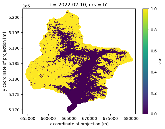
Visualize one time step of the timeseries#
Let’s download the whole image time series as a netcdf file to have a look how our first results look like
snowmap_cloudfree_1d = snowmap_cloudfree_masked.filter_temporal('2022-02-10', '2022-02-12')
snowmap_cloudfree_1d.download('results/snowmap_cloudfree_1d.nc')
xr.open_dataarray('results/snowmap_cloudfree_1d.nc',decode_coords="all")[0].plot.imshow()
<matplotlib.image.AxesImage at 0x2a1cba4d390>
Calculate Catchment Statistics#
We are looking at a region over time. We need to make sure that the information content meets our expected quality. Therefore, we calculate the cloud percentage for the catchment for each timestep. We use this information to filter the timeseries. All timesteps that have a cloud coverage of over 25% will be discarded.
Ultimately we are interested in the snow covered area (SCA) within the catchment. We count all snow covered pixels within the catchment for each time step. Multiplied by the pixel size that would be the snow covered area. Divided the pixel count by the total number of pixels in the catchment is the percentage of pixels covered with snow. We will use this number.
Get number of pixels in catchment: total, clouds, snow.
# number of all pixels
n_catchment = ((snowmap_cloudfree > -1) * 1.0).add_dimension(name="bands",type="bands",label="n_catchment")

# number of cloud pixels (no function needed, mask already created before)
n_cloud = cloud_mask.add_dimension(name="bands",type="bands",label="n_cloud")

# number of snow pixels
n_snow = ((snowmap_cloudfree == 1) * 1.0).add_dimension(name="bands",type="bands",label="n_snow")

# combine the binary data cubes into one data cube
n_catchment_cloud_snow = n_catchment.merge_cubes(n_cloud).merge_cubes(n_snow)

# aggregate to catchment
n_pixels = n_catchment_cloud_snow.aggregate_spatial(geometries = catchment_outline['geometry'][0], reducer = 'sum')
n_pixels
Create batch job to start processing on the backend.
# Create a batch job
n_pixels_json = n_pixels.save_result(format="JSON")
job = n_pixels_json.create_job(title="n_pixels_json")
job.start_job()
job.status()
'finished'
if job.status() == "finished":
    results = job.get_results()
    results.download_files("results_openeo_platform/")
Load the result. It contains the number of pixels in the catchment, clouds and snow.
We can calculate the percentages of cloud and snow pixels in the catchment.
with open("results_openeo_platform/timeseries.json","r") as file:
    n_pixels_json = json.load(file)
# check the first 5 entries
list(n_pixels_json.items())[:3] # careful unsorted dates due to JSON format
[('2022-03-09T00:00:00Z', [[4201607.0, 24.0, 1932487.0]]),
 ('2022-03-12T00:00:00Z', [[4201607.0, 3377768.0, 588345.0]]),
 ('2022-04-08T00:00:00Z', [[4166981.0, 3649978.0, 121573.0]])]
# Create a Pandas DataFrame to contain the values
dates = [k for k in n_pixels_json]
n_catchment_vals = [n_pixels_json[k][0][0] for k in n_pixels_json]
n_cloud_vals = [n_pixels_json[k][0][1] for k in n_pixels_json]
n_snow_vals = [n_pixels_json[k][0][2] for k in n_pixels_json]

data = {
        "time":pd.to_datetime(dates),
        "n_catchment_vals":n_catchment_vals,
        "n_cloud_vals":n_cloud_vals,
        "n_snow_vals":n_snow_vals
       }
df = pd.DataFrame(data=data).set_index("time")
# Sort the values by date
df = df.sort_values(axis=0,by="time")
df[:3]
| n_catchment_vals | n_cloud_vals | n_snow_vals | |
|---|---|---|---|
| time | |||
| 2022-02-02 00:00:00+00:00 | NaN | 4201607.0 | NaN |
| 2022-02-05 00:00:00+00:00 | 4201607.0 | 857590.0 | 2160594.0 |
| 2022-02-07 00:00:00+00:00 | 4166981.0 | 4023172.0 | 152057.0 |
Divide the number of cloudy pixels by the number of total pixels = cloud percentage
perc_cloud = df["n_cloud_vals"].values / df["n_catchment_vals"].values * 100
df["perc_cloud"] = perc_cloud
df[:3]
| n_catchment_vals | n_cloud_vals | n_snow_vals | perc_cloud | |
|---|---|---|---|---|
| time | ||||
| 2022-02-02 00:00:00+00:00 | NaN | 4201607.0 | NaN | NaN |
| 2022-02-05 00:00:00+00:00 | 4201607.0 | 857590.0 | 2160594.0 | 20.411000 |
| 2022-02-07 00:00:00+00:00 | 4166981.0 | 4023172.0 | 152057.0 | 96.548844 |
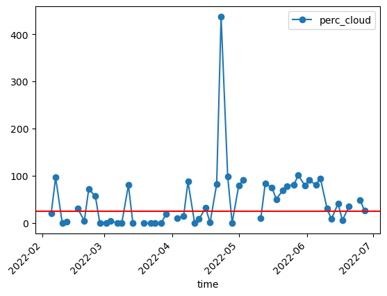
Plot the timeseries and the cloud threshold of 25%. If the cloud cover is higher the timestep will be excluded later on.
Plot the cloud percentage with the threshold.
df.plot(y="perc_cloud",rot=45,kind="line",marker='o')
plt.axhline(y = 25, color = "r", linestyle = "-")
plt.show()
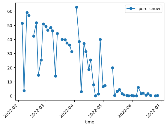
Divide the number of snow pixels by the number of total pixels = snow percentage
perc_snow = df["n_snow_vals"].values / df["n_catchment_vals"].values * 100
df["perc_snow"] = perc_snow
df[:3]
| n_catchment_vals | n_cloud_vals | n_snow_vals | perc_cloud | perc_snow | |
|---|---|---|---|---|---|
| time | |||||
| 2022-02-02 00:00:00+00:00 | NaN | 4201607.0 | NaN | NaN | NaN |
| 2022-02-05 00:00:00+00:00 | 4201607.0 | 857590.0 | 2160594.0 | 20.411000 | 51.423039 |
| 2022-02-07 00:00:00+00:00 | 4166981.0 | 4023172.0 | 152057.0 | 96.548844 | 3.649093 |
Plot the unfiltered snow percentage
df.plot(y="perc_snow",rot=45,kind="line",marker='o')
plt.show()
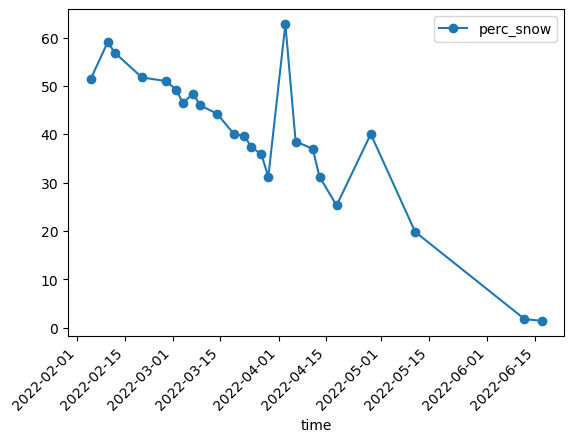
Keep only the dates with cloud coverage less than the threshold
df_filtered = df.loc[df["perc_cloud"]<25]
Plot the cloud filtered snow percentage
df_filtered.plot(y="perc_snow",rot=45,kind="line",marker='o')
plt.show()
Save the cloud filtered snow percentage
df_filtered.to_csv("results_openeo_platform/filtered_snow_perc.csv")