This notebook demonstrates with mathematical certainty that regular latitude-longitude grids introduce systematic bias in biodiversity metrics, while equal-area DGGS grids do not.
The experiment
Generate a uniform random distribution of species occurrences on the sphere (equal probability per unit area everywhere)
Count occurrences per cell on a regular lat-lon grid
Count occurrences per cell on a HEALPix DGGS grid
Compare raw counts and density estimates
Since the distribution is uniform, the true density is the same everywhere. Any variation is a grid artefact.
import numpy as np
import healpy as hp
import matplotlib.pyplot as plt

np.random.seed(42)
Step 1: Generate uniform random points on the sphere
We generate 1,000,000 random species occurrence points uniformly distributed on the sphere. This is our ground truth: density is the same everywhere.
N_POINTS = 1_000_000

# Uniform random points on the sphere
cos_theta = np.random.uniform(-1, 1, N_POINTS)
theta = np.arccos(cos_theta)
phi = np.random.uniform(0, 2 * np.pi, N_POINTS)

# Convert to latitude/longitude in degrees
lat = 90.0 - np.degrees(theta)
lon = np.degrees(phi)
lon[lon > 180] -= 360

print(f"Generated {N_POINTS:,} uniform random points on the sphere")
Generated 1,000,000 uniform random points on the sphere
Step 2: Count on a regular lat-lon grid
We use a 5-degree regular grid. Each cell spans 5 degrees in latitude and longitude. But the area of these cells varies dramatically with latitude due to meridian convergence.
GRID_RES = 5  # degrees
lat_edges = np.arange(-90, 90 + GRID_RES, GRID_RES)
lon_edges = np.arange(-180, 180 + GRID_RES, GRID_RES)
lat_centers = (lat_edges[:-1] + lat_edges[1:]) / 2
lon_centers = (lon_edges[:-1] + lon_edges[1:]) / 2

# Count occurrences per cell
counts_regular, _, _ = np.histogram2d(lat, lon, bins=[lat_edges, lon_edges])

# Compute cell areas in km²
R = 6371  # Earth radius
cell_areas = np.zeros_like(counts_regular)
for i, (lat_s, lat_n) in enumerate(zip(lat_edges[:-1], lat_edges[1:])):
    area = (
        2 * np.pi * R**2
        * abs(np.sin(np.radians(lat_n)) - np.sin(np.radians(lat_s)))
        * (GRID_RES / 360)
    )
    cell_areas[i, :] = area

print(f"Regular grid: {counts_regular.shape[0]} x {counts_regular.shape[1]} = {counts_regular.size} cells")
print(f"Cell area at equator (0°):   {cell_areas[len(lat_centers)//2, 0]:>10,.0f} km²")
print(f"Cell area at 60°:            {cell_areas[int((60+90)/GRID_RES), 0]:>10,.0f} km²")
print(f"Cell area at 85°:            {cell_areas[int((85+90)/GRID_RES), 0]:>10,.0f} km²")
print(f"Ratio equator/85°:           {cell_areas[len(lat_centers)//2, 0] / cell_areas[int((85+90)/GRID_RES), 0]:>10.1f}x")
Regular grid: 36 x 72 = 2592 cells
Cell area at equator (0°): 308,716 km²
Cell area at 60°: 142,685 km²
Cell area at 85°: 13,479 km²
Ratio equator/85°: 22.9x
Step 3: Count on a HEALPix DGGS grid
HEALPix divides the sphere into equal-area cells. Every cell has exactly the same area, regardless of latitude.
NSIDE = 16
NPIX = hp.nside2npix(NSIDE)

# Convert lat/lon to HEALPix pixel indices
pixel_indices = hp.ang2pix(NSIDE, theta, phi, nest=True)

# Count occurrences per pixel
counts_healpix = np.bincount(pixel_indices, minlength=NPIX)

# All HEALPix cells have the same area
healpix_cell_area = 4 * np.pi * R**2 / NPIX

print(f"HEALPix grid: {NPIX} cells (nside={NSIDE})")
print(f"Cell area (ALL cells): {healpix_cell_area:,.0f} km²")
print(f"Expected count per cell: {N_POINTS / NPIX:.0f}")
HEALPix grid: 3072 cells (nside=16)
Cell area (ALL cells): 166,037 km²
Expected count per cell: 326
Step 4: The key comparison — raw counts per cell
Many biodiversity studies count species occurrences per grid cell and treat each cell as equivalent. On a regular grid, this is fundamentally wrong because cells have different areas.
Let’s plot raw counts per cell by latitude. For uniform data, counts should be proportional to cell area. On the regular grid, equatorial cells are much larger → more counts. On HEALPix, all cells are the same size → counts are uniform.
fig, axes = plt.subplots(1, 2, figsize=(14, 5))

# Regular grid: mean raw count per latitude band
mean_counts_by_lat = np.mean(counts_regular, axis=1)
axes[0].bar(lat_centers, mean_counts_by_lat, width=4.5, color="tab:red", alpha=0.7)
axes[0].set_title("Regular lat-lon grid (5°)", fontsize=13)
axes[0].set_xlabel("Latitude")
axes[0].set_ylabel("Mean raw count per cell")
axes[0].axhline(N_POINTS / counts_regular.size, color="black", linestyle="--",
                label=f"If equal area: {N_POINTS / counts_regular.size:.0f}")
axes[0].legend()

# HEALPix: mean raw count per latitude band
healpix_thetas, _ = hp.pix2ang(NSIDE, np.arange(NPIX), nest=True)
healpix_lats = 90.0 - np.degrees(healpix_thetas)

lat_band_edges = np.arange(-90, 95, 5)
hp_means = []
hp_lat_centers = []
for i in range(len(lat_band_edges) - 1):
    mask = (healpix_lats >= lat_band_edges[i]) & (healpix_lats < lat_band_edges[i + 1])
    if mask.sum() > 0:
        hp_means.append(np.mean(counts_healpix[mask]))
        hp_lat_centers.append((lat_band_edges[i] + lat_band_edges[i + 1]) / 2)

axes[1].bar(hp_lat_centers, hp_means, width=4.5, color="tab:blue", alpha=0.7)
axes[1].set_title("HEALPix DGGS (nside=16)", fontsize=13)
axes[1].set_xlabel("Latitude")
axes[1].set_ylabel("Mean raw count per cell")
axes[1].axhline(N_POINTS / NPIX, color="black", linestyle="--",
                label=f"Expected: {N_POINTS / NPIX:.0f}")
axes[1].legend()

fig.suptitle(
    "Raw counts per cell for UNIFORM random data\n"
    "(uniform data should give equal counts if cells have equal area)",
    fontsize=13, fontweight="bold",
)
plt.tight_layout()
plt.savefig("../images/raw_counts_by_latitude.png", dpi=150, bbox_inches="tight")
plt.show()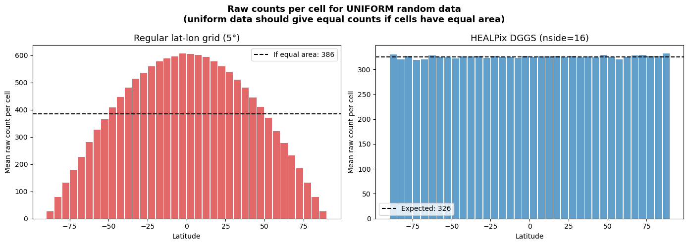
Step 5: The distortion in numbers
How much does the regular grid distort apparent species richness?
print("=" * 60)
print("REGULAR LAT-LON GRID: raw counts vary with latitude")
print("=" * 60)
print(f"  Equator (0°):  {np.mean(counts_regular[len(lat_centers)//2, :]):>6.0f} counts/cell")
print(f"  Mid-lat (45°): {np.mean(counts_regular[int((45+90)/GRID_RES), :]):>6.0f} counts/cell")
print(f"  High-lat (70°):{np.mean(counts_regular[int((70+90)/GRID_RES), :]):>6.0f} counts/cell")
print(f"  Polar (85°):   {np.mean(counts_regular[int((85+90)/GRID_RES), :]):>6.0f} counts/cell")
print()
equator_count = np.mean(counts_regular[len(lat_centers)//2, :])
polar_count = np.mean(counts_regular[int((85+90)/GRID_RES), :])
print(f"  Equator has {equator_count/polar_count:.0f}x more counts than 85° —")
print(f"  but the TRUE density is identical everywhere!")
print()
print("=" * 60)
print("HEALPIX DGGS: raw counts are uniform")
print("=" * 60)
print(f"  Mean count per cell:  {np.mean(counts_healpix):.0f}")
print(f"  Std count per cell:   {np.std(counts_healpix):.0f}")
print(f"  Coeff. of variation:  {np.std(counts_healpix)/np.mean(counts_healpix)*100:.1f}%")
print(f"  No latitude dependence — counts reflect true density.")
============================================================
REGULAR LAT-LON GRID: raw counts vary with latitude
============================================================
Equator (0°): 605 counts/cell
Mid-lat (45°): 411 counts/cell
High-lat (70°): 186 counts/cell
Polar (85°): 27 counts/cell
Equator has 22x more counts than 85° —
but the TRUE density is identical everywhere!
============================================================
HEALPIX DGGS: raw counts are uniform
============================================================
Mean count per cell: 326
Std count per cell: 19
Coeff. of variation: 5.7%
No latitude dependence — counts reflect true density.
Step 6: Map view — raw counts on both grids
The most intuitive way to see the bias: a global map of raw counts per cell. For uniform data, the map should be a single colour everywhere. Any spatial pattern is a grid artefact.
import cartopy.crs as ccrs

fig, axes = plt.subplots(
    2, 1, figsize=(14, 10),
    subplot_kw={"projection": ccrs.Robinson()},
)

# Regular grid map
lon_grid, lat_grid = np.meshgrid(lon_centers, lat_centers)
vmin = 0
vmax = np.percentile(counts_regular, 95)

shared_vmax = max(np.percentile(counts_regular, 95), np.percentile(counts_healpix, 95))

im0 = axes[0].pcolormesh(
    lon_edges, lat_edges, counts_regular,
    transform=ccrs.PlateCarree(),
    cmap="viridis", vmin=0, vmax=shared_vmax,
)
axes[0].coastlines(linewidth=0.5, color="grey")
axes[0].set_global()
axes[0].set_title("Regular lat-lon grid — raw counts per cell", fontsize=13)
plt.colorbar(im0, ax=axes[0], orientation="horizontal", pad=0.05,
             label="Count per cell", shrink=0.6)

# HEALPix map
# Use healpy mollview to create the map data, then plot manually
hp.mollview(counts_healpix, title="", hold=False, fig=None, nest=True)
plt.close()  # close healpy's figure

# Plot HEALPix as a projected map using cartopy
# Convert HEALPix to a regular grid for plotting
nside_plot = NSIDE
npix_plot = hp.nside2npix(nside_plot)
plot_lons = np.linspace(-180, 180, 720)
plot_lats = np.linspace(-90, 90, 360)
plot_lon_grid, plot_lat_grid = np.meshgrid(plot_lons, plot_lats)

# Convert lat/lon to HEALPix indices
plot_theta = np.radians(90.0 - plot_lat_grid)
plot_phi = np.radians(plot_lon_grid % 360)
plot_pix = hp.ang2pix(nside_plot, plot_theta, plot_phi, nest=True)
healpix_map = counts_healpix[plot_pix]

im1 = axes[1].pcolormesh(
    plot_lons, plot_lats, healpix_map,
    transform=ccrs.PlateCarree(),
    cmap="viridis", vmin=0, vmax=shared_vmax,
)
axes[1].coastlines(linewidth=0.5, color="grey")
axes[1].set_global()
axes[1].set_title("HEALPix DGGS — raw counts per cell", fontsize=13)
plt.colorbar(im1, ax=axes[1], orientation="horizontal", pad=0.05,
             label="Count per cell", shrink=0.6)

fig.suptitle(
    "Raw counts per cell for UNIFORM random data\n"
    "(uniform data should produce a uniform map — any pattern is a grid artefact)",
    fontsize=14, fontweight="bold", y=1.02,
)
plt.tight_layout()
plt.savefig("../images/map_raw_counts.png", dpi=150, bbox_inches="tight")
plt.show()
/home/runner/micromamba/envs/dggs-biodiversity-bias/lib/python3.11/site-packages/cartopy/io/__init__.py:241: DownloadWarning: Downloading: https://naturalearth.s3.amazonaws.com/110m_physical/ne_110m_coastline.zip
warnings.warn(f'Downloading: {url}', DownloadWarning)
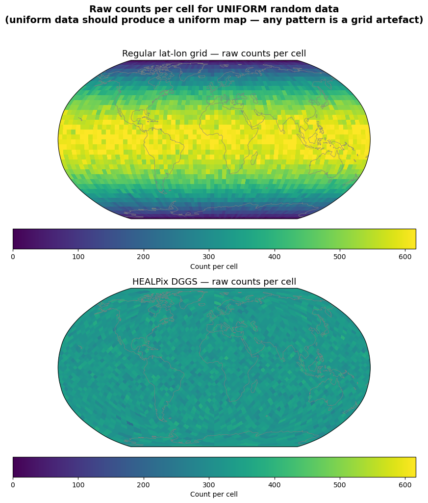
Conclusion
With uniform random data (same density everywhere on Earth):
Regular lat-lon grid: raw counts per cell vary by up to an order of magnitude with latitude because cell areas shrink toward the poles. The map shows a clear gradient from equator (high counts) to poles (low counts) — a pure grid artefact.
HEALPix DGGS: all cells have equal area. Raw counts are uniform across the globe. The map shows no spatial pattern — exactly what we expect for uniform data.
This is not a modelling result — it is a mathematical property of the grid geometry. Any biodiversity analysis on a regular grid that uses raw counts inherits this distortion.
In the next notebook, we test whether this manifests in real GBIF species occurrence data.