Part 5: Lat-lon vs Behrmann vs HEALPix — the honest 3-way comparison

Part 1 contrasted lat-lon with HEALPix. That comparison is fair as far as it goes, but it understates the case for DGGS, because the established standard for global biodiversity maps is not lat-lon raw counts — it is an equal-area cylindrical projection (Behrmann or Mollweide) applied before binning. Equal-area projections already solve the count-bias problem.

So the honest synthetic comparison shows three panels, all of 1,000,000 uniform random points on the sphere:

Lat-lon 5° grid — raw counts: a fake equator-pole gradient appears (from Part 1). This is the failure mode the audience already rejects.
Behrmann (cylindrical equal-area) grid — same data, binned in Behrmann projected space with cells of constant projected area. Cell counts are uniform across the sphere. Behrmann fixes the count bias.
HEALPix DGGS (nside=16) — same data, binned on HEALPix. Also uniform.

The slide message: equal-area projections and DGGS both pass the count test. The difference between Behrmann and HEALPix is elsewhere (cell shape, multi-resolution, ML-readiness — see Part 4).

import cartopy.crs as ccrs
import healpy as hp
import matplotlib.pyplot as plt
import numpy as np

R = 6371.0
DEG = np.pi / 180.0
np.random.seed(42)

Step 1: 1,000,000 uniform random points on the sphere¶

Same construction as Part 1: cos(θ) uniform in [-1, 1] gives uniform area density on the sphere. By construction, every grid cell with equal area on the sphere should hold the same expected count.

N_POINTS = 1_000_000
cos_theta = np.random.uniform(-1, 1, N_POINTS)
theta = np.arccos(cos_theta)
phi = np.random.uniform(0, 2 * np.pi, N_POINTS)
lat = 90.0 - np.degrees(theta)
lon = np.degrees(phi)
lon[lon > 180] -= 360
print(f"Generated {N_POINTS:,} points")

Generated 1,000,000 points

Step 2: Lat-lon 5° binning¶

Same as Part 1: cell area shrinks toward the poles, so raw counts inflate at the equator (~606 / cell at 0–5°N) and shrink toward the poles (~26 / cell at 85–90°N), purely from grid geometry.

GRID_RES = 5.0
lat_edges = np.arange(-90, 90 + GRID_RES, GRID_RES)
lon_edges = np.arange(-180, 180 + GRID_RES, GRID_RES)
counts_latlon, _, _ = np.histogram2d(lat, lon, bins=[lat_edges, lon_edges])
print(f"Lat-lon grid: {counts_latlon.shape}, total {int(counts_latlon.sum()):,}")

Lat-lon grid: (36, 72), total 1,000,000

Step 3: Behrmann (cylindrical equal-area) binning¶

Behrmann projection (standard parallels ±30°):

x = R · λ · cos(30°)        y = R · sin(φ) / cos(30°)

A grid that is regular in Behrmann projected space has cells of constant area on the sphere — that is the defining property of an equal-area projection. We size the Behrmann cell to match the HEALPix nside=16 cell area (~166,000 km²). That way the two equal-area panels read the same colour on a shared scale and only the lat-lon panel shows a spatial pattern.

# Behrmann projected coordinates of every point
x_proj = R * (lon * DEG) * np.cos(30 * DEG)
y_proj = R * np.sin(lat * DEG) / np.cos(30 * DEG)

# Match HEALPix nside=16 cell area exactly: 4πR² / 3072 ≈ 166,000 km².
# A square Behrmann projected cell of side s has cell area s². So:
HEALPIX_AREA_KM2 = 4 * np.pi * R**2 / (12 * 16**2)
dx = np.sqrt(HEALPIX_AREA_KM2)
dy = np.sqrt(HEALPIX_AREA_KM2)

# Number of cells along each Behrmann projected axis
x_min = R * (-180.0 * DEG) * np.cos(30 * DEG)
x_max = R * (180.0 * DEG) * np.cos(30 * DEG)
y_min = R * np.sin(-90 * DEG) / np.cos(30 * DEG)
y_max = R * np.sin(90 * DEG) / np.cos(30 * DEG)

n_x = int(np.round((x_max - x_min) / dx))
n_y = int(np.round((y_max - y_min) / dy))
behrmann_x_edges = np.linspace(x_min, x_max, n_x + 1)
behrmann_y_edges = np.linspace(y_min, y_max, n_y + 1)

counts_behrmann, _, _ = np.histogram2d(
    y_proj, x_proj, bins=[behrmann_y_edges, behrmann_x_edges]
)
print(f"Behrmann grid: {counts_behrmann.shape}, total {int(counts_behrmann.sum()):,}")

Behrmann grid: (36, 85), total 1,000,000

Step 4: HEALPix nside=16 binning¶

Same as Part 1.

NSIDE = 16
NPIX = hp.nside2npix(NSIDE)
pix = hp.ang2pix(NSIDE, theta, phi, nest=True)
counts_healpix = np.bincount(pix, minlength=NPIX)
print(f"HEALPix grid: nside={NSIDE}, NPIX={NPIX}")
print(f"  mean count/cell: {counts_healpix.mean():.1f}")
print(f"  std  count/cell: {counts_healpix.std():.1f}")

HEALPix grid: nside=16, NPIX=3072
  mean count/cell: 325.5
  std  count/cell: 18.6

Step 5: Compare all three on the same Mollweide display¶

Each grid’s count field is sampled onto a fine plotting raster (Mollweide display lat/lon → grid index → count) so all three panels share the same display projection and the same colour scale. The colour scale spans 0 to the lat-lon equator-band peak so the lat-lon failure mode is visible.

plot_n_lon, plot_n_lat = 720, 360
plot_lons = np.linspace(-180, 180, plot_n_lon)
plot_lats = np.linspace(-90, 90, plot_n_lat)
LON, LAT = np.meshgrid(plot_lons, plot_lats)

# Lat-lon raster
i_lat = np.clip(((LAT - lat_edges[0]) / GRID_RES).astype(int),
                0, counts_latlon.shape[0] - 1)
i_lon = np.clip(((LON - lon_edges[0]) / GRID_RES).astype(int),
                0, counts_latlon.shape[1] - 1)
field_latlon = counts_latlon[i_lat, i_lon]

# Behrmann raster
xp = R * (LON * DEG) * np.cos(30 * DEG)
yp = R * np.sin(LAT * DEG) / np.cos(30 * DEG)
i_y = np.clip(((yp - y_min) / dy).astype(int), 0, n_y - 1)
i_x = np.clip(((xp - x_min) / dx).astype(int), 0, n_x - 1)
field_behrmann = counts_behrmann[i_y, i_x]

# HEALPix raster
plot_theta = np.radians(90.0 - LAT)
plot_phi = np.radians(LON % 360)
plot_pix = hp.ang2pix(NSIDE, plot_theta, plot_phi, nest=True)
field_healpix = counts_healpix[plot_pix]

# Shared colour scale: cap at the lat-lon equator-band peak so the
# bias is visible on panel 1 and panels 2/3 both read as ~uniform.
shared_vmax = float(np.percentile(field_latlon, 99))

panels = [
    ("Lat-lon 5° × 5°  —  raw counts per cell\n"
     "(equator-pole gradient is pure grid artefact)",
     field_latlon),
    ("Behrmann (cylindrical equal-area)  —  raw counts per cell\n"
     "(established biodiversity standard — uniform, as expected)",
     field_behrmann),
    (f"HEALPix DGGS (nside={NSIDE})  —  raw counts per cell\n"
     "(also uniform — equal-area without a projection)",
     field_healpix),
]

fig = plt.figure(figsize=(12, 13))
gs = fig.add_gridspec(3, 1, hspace=0.35)

for row, (title, field) in enumerate(panels):
    ax = fig.add_subplot(gs[row, 0], projection=ccrs.Mollweide())
    im = ax.pcolormesh(
        plot_lons, plot_lats, field,
        transform=ccrs.PlateCarree(), cmap="viridis",
        vmin=0, vmax=shared_vmax,
    )
    ax.coastlines(linewidth=0.4, color="0.45")
    ax.set_global()
    ax.set_title(title, fontsize=11)

cbar_ax = fig.add_axes([0.15, 0.05, 0.7, 0.018])
fig.colorbar(im, cax=cbar_ax, orientation="horizontal",
             label="Count per cell")

fig.suptitle(
    "1,000,000 uniformly-distributed points on the sphere — "
    "same data, three grids",
    fontsize=14, fontweight="bold", y=0.99,
)
fig.text(
    0.5, 0.015,
    "Behrmann and HEALPix both solve the count bias. "
    "The difference between them shows up in cell shape (see kernel-footprint figure).",
    ha="center", va="bottom", fontsize=10, style="italic", color="0.25",
)

plt.savefig("../images/equal_area_comparison.png", dpi=150, bbox_inches="tight")
plt.show()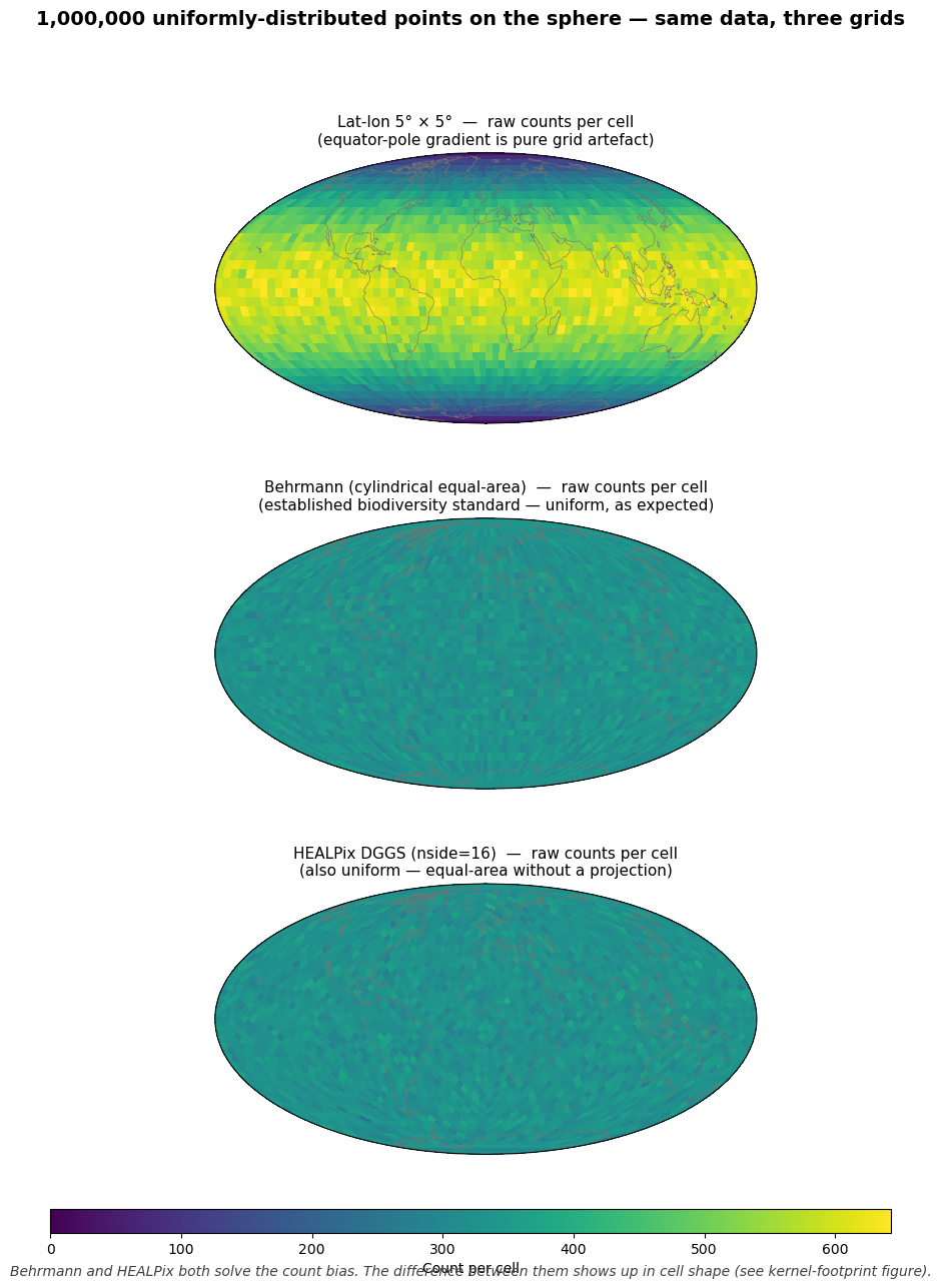

What the figure shows¶

Top. Lat-lon raw counts for uniform data show a fake equator- pole gradient. This is the failure mode of the most-naive grid.

Middle. Behrmann projected cells are equal-area on the sphere by construction; counts are uniform. Behrmann (and Mollweide, Lambert cylindrical equal-area, etc.) is the recognized standard for global biodiversity maps for exactly this reason.

Bottom. HEALPix nside=16 cells are also equal-area; counts are also uniform.

The slide-5 setup. Behrmann and HEALPix both pass the count test — equal-area is a solved problem and the audience already accepts the equal-area requirement. The interesting question is what comes after equal-area: cell shape, multi-resolution, cloud-native indexing. That argument is made by the kernel- footprint figure (Part 4).