Part 6: Hierarchical indexing in HEALPix (NESTED ordering)

A practical advantage of DGGS over equal-area projections is hierarchical refinement without reprojection. In HEALPix’s NESTED ordering, every cell at resolution nside = N has exactly 4 children at resolution nside = 2N, and the parent’s cell index is the prefix of the child’s index in base-4. Refining from coarse to fine is a bit-shift, not a re-binning of data.

This is the feature that makes DGGS multi-resolution and cloud- native: the same global stack can be aggregated to coarse cells (e.g. for fast continental-scale analysis) or refined to fine cells (e.g. for habitat patches near a research station) without ever re-projecting or re-resampling the underlying data.

This notebook visualises that hierarchy at three resolutions over Scandinavia, the same region used in Part 4.

import cartopy.crs as ccrs
import cartopy.feature as cfeature
import healpy as hp
import matplotlib.pyplot as plt
import numpy as np

R = 6371.0
DEG = np.pi / 180.0

ANCHOR_LAT = 65.0
ANCHOR_LON = 15.0
DISPLAY_HALF_EXTENT_KM = 1500e3

Pick a parent cell at the coarsest level, then walk its tree¶

We start at nside = 8 (768 cells globally, ~664,000 km² each), pick the cell that contains (65°N, 15°E), and walk its quadtree down to nside = 32 (16 children) and nside = 128 (256 great-grandchildren). The parent–child relationship is entirely encoded in the NESTED index: refining nside by 2× turns each parent index p into children 4p, 4p+1, 4p+2, 4p+3.

def nested_descendants(parent_pix, parent_nside, target_nside):
    """All NESTED pixel indices at `target_nside` that descend from
    `parent_pix` at `parent_nside`. Refinement factor must be a
    power of 2."""
    factor = target_nside // parent_nside
    assert (factor & (factor - 1)) == 0, "factor must be a power of 2"
    levels = int(np.log2(factor))
    children = np.array([parent_pix], dtype=np.int64)
    for _ in range(levels):
        children = np.concatenate([4 * children + k for k in range(4)])
    return children


def cell_outline(nside, pix, step=8, nest=True):
    """Return cell boundary as (lat, lon) arrays."""
    xyz = hp.boundaries(nside, pix, step=step, nest=nest)
    x, y, z = xyz
    lats = 90.0 - np.degrees(np.arccos(z))
    lons = np.degrees(np.arctan2(y, x))
    return lats, lons


# Parent at nside=8 containing the anchor
PARENT_NSIDE = 8
theta_a = (90.0 - ANCHOR_LAT) * DEG
phi_a = (ANCHOR_LON % 360) * DEG
parent_pix = hp.ang2pix(PARENT_NSIDE, theta_a, phi_a, nest=True)
print(f"NESTED parent index at nside={PARENT_NSIDE}: {parent_pix}")
print(f"  area: {4 * np.pi * R**2 / hp.nside2npix(PARENT_NSIDE):,.0f} km²")

# Children at nside=32 (16 of them)
CHILD_NSIDE = 32
children = nested_descendants(parent_pix, PARENT_NSIDE, CHILD_NSIDE)
print(f"\n{len(children)} NESTED children at nside={CHILD_NSIDE}:")
print(f"  indices {children[0]} … {children[-1]}")
print(f"  area:   {4 * np.pi * R**2 / hp.nside2npix(CHILD_NSIDE):,.0f} km² each")

# Grand-grandchildren at nside=128 (256 of them)
GC_NSIDE = 128
grandchildren = nested_descendants(parent_pix, PARENT_NSIDE, GC_NSIDE)
print(f"\n{len(grandchildren)} NESTED descendants at nside={GC_NSIDE}:")
print(f"  area: {4 * np.pi * R**2 / hp.nside2npix(GC_NSIDE):,.0f} km² each")

NESTED parent index at nside=8: 58
  area: 664,146 km²

16 NESTED children at nside=32:
  indices 928 … 943
  area:   41,509 km² each

256 NESTED descendants at nside=128:
  area: 2,594 km² each

Build the figure¶

A single panel: same parent cell at three resolutions, all overlaid. The parent cell at nside=8 is outlined boldly. Inside it, the 16 children at nside=32 are drawn with medium contrast. Inside those, the 256 great-grandchildren at nside=128 are drawn with light contrast. Every finer grid is exactly nested inside the coarser one — the coarse boundary is also a fine boundary, no resampling.

display_proj = ccrs.LambertAzimuthalEqualArea(
    central_latitude=ANCHOR_LAT, central_longitude=ANCHOR_LON
)

fig = plt.figure(figsize=(11, 9))
ax = fig.add_subplot(1, 1, 1, projection=display_proj)
ax.set_extent(
    [-DISPLAY_HALF_EXTENT_KM, DISPLAY_HALF_EXTENT_KM,
     -DISPLAY_HALF_EXTENT_KM, DISPLAY_HALF_EXTENT_KM],
    crs=display_proj,
)
ax.add_feature(cfeature.LAND, facecolor="0.94")
ax.add_feature(cfeature.OCEAN, facecolor="0.97")
ax.coastlines(linewidth=0.5, color="0.4")
ax.gridlines(linewidth=0.3, color="0.7", alpha=0.6)

# Fill the parent territory in pale orange so the boundary of the
# whole nested region is unmistakable on the map.
parent_lats, parent_lons = cell_outline(PARENT_NSIDE, parent_pix)
ax.fill(parent_lons, parent_lats, transform=ccrs.PlateCarree(),
        facecolor="tab:orange", alpha=0.18, zorder=2)

# Finest grid: 256 great-grandchildren at nside=128, light grey.
for pix in grandchildren:
    lats, lons = cell_outline(GC_NSIDE, pix, step=4)
    ax.plot(lons, lats, transform=ccrs.PlateCarree(),
            color="0.55", linewidth=0.45, alpha=0.85, zorder=3)

# Middle grid: 16 children at nside=32, medium contrast.
for pix in children:
    lats, lons = cell_outline(CHILD_NSIDE, pix, step=8)
    ax.plot(lons, lats, transform=ccrs.PlateCarree(),
            color="tab:blue", linewidth=1.4, alpha=0.95, zorder=4)

# Coarsest grid: parent boundary at nside=8, bold.
ax.plot(parent_lons, parent_lats, transform=ccrs.PlateCarree(),
        color="tab:orange", linewidth=3.0, alpha=1.0, zorder=5)

# Anchor point
ax.plot(ANCHOR_LON, ANCHOR_LAT, marker="o", markersize=8,
        markerfacecolor="black", markeredgecolor="white",
        markeredgewidth=1.5, transform=ccrs.PlateCarree(), zorder=6)

# Inline legend (manual, so we control colours and weights)
from matplotlib.lines import Line2D
legend_handles = [
    Line2D([0], [0], color="tab:orange", linewidth=3.0,
           label=f"nside={PARENT_NSIDE}  ·  1 parent cell  ·  ~664·10³ km²"),
    Line2D([0], [0], color="tab:blue", linewidth=1.4,
           label=f"nside={CHILD_NSIDE}  ·  16 children   ·  ~42·10³ km²"),
    Line2D([0], [0], color="0.55", linewidth=0.6,
           label=f"nside={GC_NSIDE}  ·  256 descendants ·  ~3·10³ km²"),
]
ax.legend(handles=legend_handles, loc="lower left", fontsize=10,
          framealpha=0.95, title="HEALPix NESTED — same region, three resolutions",
          title_fontsize=10)

ax.set_title(
    "Hierarchical refinement in HEALPix (NESTED) — "
    "every finer grid is exactly nested inside the coarser one",
    fontsize=12, fontweight="bold",
)
fig.text(
    0.5, 0.04,
    f"Parent index {parent_pix} (nside={PARENT_NSIDE})  →  "
    f"children {{{children[0]}, …, {children[-1]}}} at nside={CHILD_NSIDE}  →  "
    f"descendants {{{grandchildren[0]}, …, {grandchildren[-1]}}} at nside={GC_NSIDE}\n"
    "Refinement is a bit-shift on the cell index — no projection, no resampling.",
    ha="center", va="bottom", fontsize=9, style="italic", color="0.25",
)

plt.savefig("../images/hierarchical_indexing.png", dpi=150, bbox_inches="tight")
plt.show()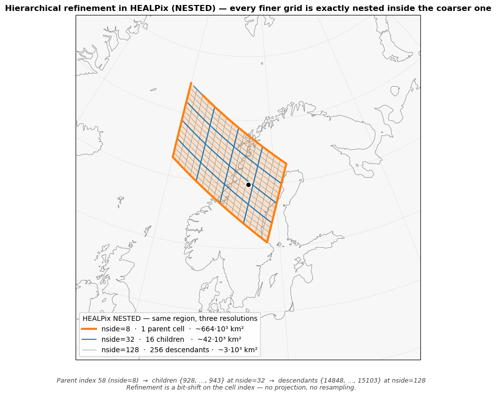

What the figure shows¶

The orange region is the same on the sphere in all three panels.

Left, nside=8. One parent cell of ~664,000 km².
Middle, nside=32. 16 children of ~41,500 km² each, exactly tiling the parent. Cell indices 4²·p + 0 … 4²·p + 15 in NESTED ordering.
Right, nside=128. 256 descendants of ~2,600 km² each, again exactly tiling the same region. Indices 4⁴·p + 0 … 4⁴·p + 255.

Refining from any level to any deeper level is a deterministic integer operation on the cell index. There is no projection step, no interpolation, no resampling artefact. A model trained on coarse-resolution features can be applied to fine-resolution cells by simply traversing the tree, and a coarse aggregate is computed by truncating bits of the fine index.

Slide-5 takeaway. Behrmann or Mollweide deliver equal-area cells but at one fixed resolution. Refining their cells requires a fresh reprojection of every input layer in the stack. HEALPix NESTED gives equal-area and a free, deterministic, multi- resolution hierarchy — the property that makes a stacked, AI-readable feature cube practical to maintain across many resolutions and many ingestion pipelines.