Notebook 07 established that all six equal-area aggregation choices (HEALPix, H3, rHEALPix, Mollweide, EEA reference grid, ISEA3H) agree on biodiversity density patterns; lat-lon is the only one that distorts. Notebooks 03 and 04 established that the DGGS family (HEALPix, H3, rHEALPix, ISEA3H) preserves compact cell shape across latitudes, while the projection family (Behrmann, Mollweide, partly EEA) does not.
So why HEALPix specifically? This notebook isolates three HEALPix-family advantages that distinguish it from the other DGGS choices and matter for climate-driven biodiversity science:
Section A — Sphere vs WGS84 ellipsoid. HEALPix is defined on the unit sphere. EO data, GBIF occurrences, and Copernicus products are referenced to the WGS84 ellipsoid. The mismatch is small (~0.7% area error at boreal latitudes) but systematic and compounding — exactly the regime where climate-driven biodiversity attribution conclusions live or die. Solutions: rHEALPix (HEALPix on WGS84 directly) and Ellipsoidal HEALPix via the authalic-sphere mapping (the GRID4EARTH approach).
Section B — NESTED bit-shift refinement. Parent and children of any HEALPix cell are computed by integer bit operations alone (parent =
pix >> 2, children =pix << 2 | k). This makes zoom-in / zoom-out O(1) per cell, with no projection, no resampling, no hash lookup.Section C — Iso-latitude pixelization. All HEALPix cells in the same “ring” share the same colatitude. This makes latitude-banded analyses (zonal extinction risk, latitudinal phenology, climate-zone aggregation) trivially fast.
Section A — HEALPix on the sphere vs HEALPix on the WGS84 ellipsoid
The Earth is not a sphere. WGS84 — the geodetic datum every Copernicus product, every GBIF occurrence, every Destination Earth climate model output uses — is an oblate ellipsoid with flattening ~1/298.26. HEALPix’s mathematics, by contrast, is defined on the unit sphere (Górski et al. 2005).
When we feed a (lat, lon) pair into hp.ang2pix(nside, theta, phi),
we are asking “which HEALPix cell does this point fall into,
treating it as if it were on a sphere?” — and the cell areas HEALPix
uses are spherical cell areas, not the area of the equivalent patch
on the WGS84 ellipsoid where the data actually lives.
The error this introduces is small — at most ~0.9% per cell at 85°N, smaller everywhere else. For biodiversity counts in isolation it is well below other sources of error (GBIF sampling effort variability, species-distribution-model uncertainty, climate-model spread). The sphere version of HEALPix is fine for straightforward biodiversity-occurrence aggregation at coarse resolution.
Where this bias becomes material is the integration regime — the future where biodiversity data is stacked at high resolution with Copernicus EO products and Destination Earth climate model output on a single common DGGS. There the bias is systematic in latitude, accumulates across products, and lives at precisions where zonal trend detection actually operates. This is precisely the regime that ESA GRID4EARTH identifies as requiring an ellipsoidally-correct common DGGS for the Copernicus × Destination Earth bridge.
This section quantifies the mismatch and shows the two existing paths that solve it for the integration regime.
import numpy as np
import matplotlib.pyplot as plt
from pyproj import Geod

WGS84 = Geod(ellps="WGS84")

# A few canonical sphere-radius choices used in HEALPix-on-sphere work:
R_MEAN_KM = 6371.0          # mean Earth radius (the "obvious" choice)
R_AUTHALIC_KM = 6371.0072   # authalic sphere — same total surface area as WGS84
R_VOLUME_KM = 6371.0008     # volume-equivalent sphere
A_WGS84_KM = 6378.137       # WGS84 semi-major axis
B_WGS84_KM = 6356.752314245 # WGS84 semi-minor axis (derived from f = 1/298.257223563)
Cell area: sphere vs WGS84 ellipsoid
We pick a 1° × 1° geodetic-coordinates cell at latitude φ (the typical biodiversity-aggregation resolution at country scale) and compute its area:
on the unit sphere (mean / authalic radius), treating geodetic lat as if it were spherical colatitude;
on the WGS84 ellipsoid, using
pyproj.Geod.polygon_area_perimeterwhich solves the geodesic exactly.
The discrepancy is what HEALPix-on-sphere systematically gets wrong.
def cell_area_sphere(lat_c, dlat=1.0, dlon=1.0, radius_km=R_MEAN_KM):
    """Area (km²) of a geodetic 1°×1° cell, treated as spherical."""
    lat_n = np.radians(lat_c + dlat / 2)
    lat_s = np.radians(lat_c - dlat / 2)
    return radius_km ** 2 * np.radians(dlon) * (np.sin(lat_n) - np.sin(lat_s))


def cell_area_wgs84(lat_c, dlat=1.0, dlon=1.0):
    """True WGS84-ellipsoidal area (km²) of a 1°×1° cell."""
    lons = [-dlon / 2, dlon / 2, dlon / 2, -dlon / 2]
    lats = [lat_c - dlat / 2, lat_c - dlat / 2,
            lat_c + dlat / 2, lat_c + dlat / 2]
    area_m2, _ = WGS84.polygon_area_perimeter(lons, lats)
    return abs(area_m2) / 1e6  # km²


lat_grid = np.linspace(0, 89, 90)
A_mean = np.array([cell_area_sphere(l, radius_km=R_MEAN_KM) for l in lat_grid])
A_authalic = np.array([cell_area_sphere(l, radius_km=R_AUTHALIC_KM) for l in lat_grid])
A_wgs84 = np.array([cell_area_wgs84(l) for l in lat_grid])

err_mean_pct = 100 * (A_mean - A_wgs84) / A_wgs84
err_authalic_pct = 100 * (A_authalic - A_wgs84) / A_wgs84

print("Sample cell-area errors (1°×1° cell, sphere vs WGS84):")
print(f"  {'lat':>5} {'A_sphere(km²)':>14} {'A_wgs84(km²)':>14} {'err_mean(%)':>12} {'err_authalic(%)':>16}")
for lat in [0, 30, 45, 65, 70, 85]:
    i = int(lat)
    print(f"  {lat:>5} {A_mean[i]:>14.1f} {A_wgs84[i]:>14.1f} "
          f"{err_mean_pct[i]:>+12.4f} {err_authalic_pct[i]:>+16.4f}")
Sample cell-area errors (1°×1° cell, sphere vs WGS84):
lat A_sphere(km²) A_wgs84(km²) err_mean(%) err_authalic(%)
0 12364.2 12309.2 +0.4462 +0.4464
30 10707.7 10695.7 +0.1122 +0.1124
45 8742.8 8762.2 -0.2212 -0.2210
65 5225.3 5259.5 -0.6491 -0.6489
70 4228.8 4259.9 -0.7310 -0.7308
85 1077.6 1087.1 -0.8764 -0.8762
Where this matters — and where it doesn’t
The maximum percentage error is small (~+0.45% at the equator, ~−0.88% at 85°N). At first glance this looks negligible compared to the count bias of lat-lon (up to 23× at 5° resolution; notebook 02).
For biodiversity counts at coarse resolution in isolation, it is negligible. It sits well below GBIF sampling-effort variability, species-distribution-model uncertainty, and climate-model spread. Sphere HEALPix is fine for typical biodiversity-occurrence aggregation, range maps, and density estimates.
For the integration regime, the structure of the error matters:
Systematic, not random. The error always has the same sign at a given latitude. It does not average out.
Latitude-dependent. The error swings ~1.3 percentage points across the populated latitude range. Zonal comparisons (boreal vs temperate vs tropical) accumulate this swing as a bias.
Cross-product accumulation. When biodiversity data is fused with Copernicus EO products and Destination Earth model output on a common grid, the per-product systematic biases compose. The integrated stack carries the union of the latitudinal biases.
Long-term trend detection. A 0.7% systematic bias in zonal density estimates is on the same order as the per-decade trends that climate-driven range-shift attribution actually targets.
This is the regime ESA GRID4EARTH identifies as requiring an ellipsoidally-correct common DGGS for the Copernicus × Destination Earth bridge — and biodiversity science integrated into that bridge inherits the requirement.
The figure — sphere-vs-WGS84 area error vs latitude
fig = plt.figure(figsize=(13, 5.5))
gs = fig.add_gridspec(1, 2, wspace=0.30)

# -- Left: cell areas in km² ----------------------------------------
ax_a = fig.add_subplot(gs[0, 0])
ax_a.plot(lat_grid, A_mean, color="tab:red", lw=2,
          label=f"Sphere R={R_MEAN_KM:.0f} km (mean radius)")
ax_a.plot(lat_grid, A_authalic, color="tab:orange", lw=1.4, linestyle="--",
          label=f"Sphere R={R_AUTHALIC_KM:.4f} km (authalic — equal total area)")
ax_a.plot(lat_grid, A_wgs84, color="tab:blue", lw=2,
          label="WGS84 ellipsoid (pyproj.Geod, exact)")
ax_a.set_xlabel("Latitude (°N)")
ax_a.set_ylabel("Cell area (km²) of a 1° × 1° geodetic cell")
ax_a.set_title("Area of a 1° × 1° cell — sphere vs WGS84 ellipsoid",
               fontsize=11, fontweight="bold")
ax_a.legend(loc="upper right", fontsize=9, framealpha=0.95)
ax_a.set_xlim(0, 89)
ax_a.grid(alpha=0.3)

# -- Right: % error vs latitude -------------------------------------
ax_b = fig.add_subplot(gs[0, 1])
ax_b.fill_between(lat_grid, 0, err_mean_pct,
                  where=err_mean_pct >= 0, color="tab:red", alpha=0.18,
                  label="Sphere-on-WGS84 over-estimates area")
ax_b.fill_between(lat_grid, 0, err_mean_pct,
                  where=err_mean_pct < 0, color="tab:blue", alpha=0.18,
                  label="Sphere-on-WGS84 under-estimates area")
ax_b.plot(lat_grid, err_mean_pct, color="tab:red", lw=2,
          label=f"Sphere R={R_MEAN_KM:.0f} km (mean)")
ax_b.plot(lat_grid, err_authalic_pct, color="tab:orange", lw=1.4,
          linestyle="--",
          label=f"Sphere R={R_AUTHALIC_KM:.2f} km (authalic)")
ax_b.axhline(0, color="0.4", linewidth=0.7)
ax_b.set_xlabel("Latitude (°N)")
ax_b.set_ylabel("(A_sphere − A_WGS84) / A_WGS84   (%)")
ax_b.set_title(
    "Systematic area error of HEALPix-on-sphere\n"
    "across the populated latitude range",
    fontsize=11, fontweight="bold",
)
ax_b.legend(loc="lower left", fontsize=8.5, framealpha=0.95)
ax_b.set_xlim(0, 89)
ax_b.grid(alpha=0.3)

# Annotation box at boreal latitudes
ax_b.annotate(
    f"At 65°N: {err_mean_pct[65]:+.3f}%\n"
    f"At 70°N: {err_mean_pct[70]:+.3f}%\n"
    f"At 85°N: {err_mean_pct[85]:+.3f}%",
    xy=(70, err_mean_pct[70]), xytext=(45, -0.4),
    fontsize=8.5, family="monospace",
    bbox=dict(boxstyle="round,pad=0.4", facecolor="white",
              edgecolor="0.6", alpha=0.95),
    arrowprops=dict(arrowstyle="->", color="0.4"),
)

fig.suptitle(
    "HEALPix-on-sphere vs HEALPix-on-WGS84 — small per-cell error, "
    "systematic across latitude, compounding for climate-biodiversity "
    "attribution",
    fontsize=12, fontweight="bold", y=1.02,
)

plt.savefig("../images/sphere_vs_ellipsoid_area_error.png",
            dpi=150, bbox_inches="tight")
plt.show()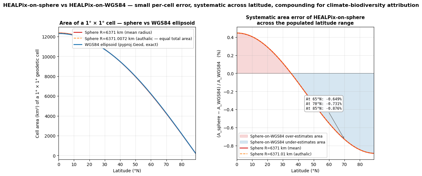
Two existing solutions
rHEALPix (already in this study). rHEALPix defines HEALPix-style
equal-area cells directly on the WGS84 ellipsoid, via a cube
projection. Cells have exactly equal area on the actual Earth shape
— no mean / authalic / volume sphere choice needed. We used
rhealpixdggs (PyPI) in notebook 07; it is the pip-installable,
production-ready answer for an ellipsoid-native HEALPix family
member.
Ellipsoidal HEALPix via authalic-sphere mapping (GRID4EARTH). The GRID4EARTH (ESA) approach is to map the WGS84 ellipsoid to its authalic sphere (the sphere with the same total surface area) via the standard authalic-latitude transform. HEALPix defined on the authalic sphere then yields cells of exactly equal area on the original WGS84 ellipsoid — preserving the equal-area property while using the well-established HEALPix code path. This bridges spherical climate models (Destination Earth) and ellipsoidal Earth-observation data (Copernicus) on a single common DGGS.
Both approaches eliminate the per-latitude ~0.7% systematic bias
documented in this section. Choosing between them is a matter of
code-base alignment: rhealpixdggs is mature and pip-installable;
Ellipsoidal HEALPix lives inside the GRID4EARTH ecosystem and is
the path that integrates with the Destination Earth Common Data
Model.
Both Section B (NESTED bit-shift) and Section C (iso-latitude) below are pure HEALPix-family properties that survive the sphere → authalic mapping unchanged.
Section B — NESTED bit-shift refinement: zoom-in / zoom-out is O(1)
In HEALPix NESTED ordering the parent–child relationship is pure integer arithmetic:
parent(pix)        = pix >> 2
children(pix, k)   = (pix << 2) | k    for k in {0, 1, 2, 3}
That means zoom in / zoom out — going between any two HEALPix
resolutions (nside = N and nside = 2N) — is O(1) per cell,
with no projection, no resampling, no hash lookup, no coordinate
conversion. For any tile-based or multi-resolution biodiversity
pipeline (Copernicus chunked Zarr × Destination Earth × GBIF stacks)
this property is what makes a HEALPix-keyed feature cube tractable
at scale.
This section verifies the bit-shift relation against healpy and
discusses the implications.
import healpy as hp

# Pick a cell at low resolution and compute its 4 children at
# the next refinement level via bit-shift.
PARENT_NSIDE = 8
CHILD_NSIDE = 2 * PARENT_NSIDE  # 16

parent_pix = 42
children_via_bitshift = [(parent_pix << 2) | k for k in range(4)]
parent_recovered = children_via_bitshift[0] >> 2

print(f"Parent (nside={PARENT_NSIDE}, NESTED):  pix = {parent_pix} = {parent_pix:08b}")
print(f"Children at nside={CHILD_NSIDE} via bit-shift:")
for k, c in enumerate(children_via_bitshift):
    print(f"  k={k}: pix = {c:>4} = {c:010b}")
print(f"Recovering parent from any child via >> 2: {parent_recovered}")
assert parent_recovered == parent_pix
Parent (nside=8, NESTED): pix = 42 = 00101010
Children at nside=16 via bit-shift:
k=0: pix = 168 = 0010101000
k=1: pix = 169 = 0010101001
k=2: pix = 170 = 0010101010
k=3: pix = 171 = 0010101011
Recovering parent from any child via >> 2: 42
Verifying via healpy: each child’s centre is geographically
inside the parent.
We get each child’s centroid (lat, lon) from hp.pix2ang(..., nest=True) and confirm that hp.ang2pix(parent_nside, ..., nest=True) returns the parent. This is a tautology of NESTED
ordering but is worth demonstrating once.
# theta is colatitude, phi is longitude in radians
child_thetas, child_phis = hp.pix2ang(
    CHILD_NSIDE, np.array(children_via_bitshift), nest=True,
)
parent_check = hp.ang2pix(PARENT_NSIDE, child_thetas, child_phis, nest=True)
print(f"hp.ang2pix(parent_nside, child_centres) = {parent_check.tolist()}")
print(f"Expected parent_pix everywhere: {parent_pix}")
assert all(p == parent_pix for p in parent_check)
hp.ang2pix(parent_nside, child_centres) = [42, 42, 42, 42]
Expected parent_pix everywhere: 42
Practical implication for biodiversity-EO stacks
A pipeline that ingests Copernicus Zarr chunks at native HEALPix
resolution and downsamples them to a coarser analysis grid for
GBIF-aggregated species-distribution modelling does not need a
resampling step in the HEALPix-NESTED case. It is a chunk index
bit-shift. For every cell at coarse nside, the four (or sixteen,
or 4^k) tiles at fine nside × 2^k are known by integer arithmetic
alone — directly addressable in the chunked store.
This is the algorithmic property that distinguishes HEALPix from
H3 and ISEA3H for tile-based / cloud-native analytics. H3 has
hierarchical refinement too, but its parent-child relation requires
a small lookup; ISEA3H’s hierarchical addressing (Z3, Z7, etc.)
also works but is again not a single instruction. NESTED HEALPix
is pix >> 2. Nothing else.
Section C — Iso-latitude pixelization: zonal analyses are trivial
In HEALPix every cell belongs to a “ring” of cells at the same
colatitude. The ring number is recoverable from the pixel index in
RING ordering directly; in NESTED ordering it is one healpy call
(hp.pix2ang) but the underlying property is the same:
All HEALPix pixels in the same ring sit at exactly the same latitude.
This makes zonal analyses — climate-zone × biodiversity stats, latitudinal phenology curves, latitudinal extinction-risk gradients — almost free. No spatial query, no polygon clipping; just group pixels by ring index.
Hexagonal DGGS (H3, ISEA3H) do not have this property: cells on the “same row” of a hex tessellation are at slightly different latitudes because hexagons do not tile latitude bands. For latitude-banded climate-biodiversity work this is a real, if subtle, advantage of HEALPix.
NSIDE_RINGS = 16

# Pick a ring at HEALPix nside=16 and confirm every pixel in the ring
# has the same latitude.
ring_idx = 12  # 0-indexed; ring 0 is at the north pole
ring_pix = hp.query_strip(NSIDE_RINGS,
                          theta1=0, theta2=np.pi,
                          inclusive=False, nest=False)
# query_strip returns all pixels in a colatitude range; for an
# iso-latitude demonstration we use ring2pix-equivalent: use the fact
# that in RING ordering, pixels are stored ring-by-ring. Equivalent:
ring_pix_in_ring = []
for pix_ring in range(hp.nside2npix(NSIDE_RINGS)):
    th, _ = hp.pix2ang(NSIDE_RINGS, pix_ring, nest=False)
    if abs(th - hp.pix2ang(NSIDE_RINGS, 12 * NSIDE_RINGS, nest=False)[0]) < 1e-10:
        ring_pix_in_ring.append(pix_ring)

# Convert back to NESTED indices for use elsewhere in the notebook
ring_pix_nest = hp.ring2nest(NSIDE_RINGS, np.array(ring_pix_in_ring))

# Confirm all pixels in the ring share the same colatitude
ring_thetas, ring_phis = hp.pix2ang(NSIDE_RINGS,
                                     np.array(ring_pix_in_ring),
                                     nest=False)
print(f"HEALPix nside={NSIDE_RINGS}: ring contains {len(ring_pix_in_ring)} pixels")
print(f"Colatitude θ of all pixels in the ring: "
      f"min={ring_thetas.min():.10f}, max={ring_thetas.max():.10f}")
print(f"Latitude    of all pixels in the ring: "
      f"{90.0 - np.degrees(ring_thetas[0]):.4f}°")
assert np.allclose(ring_thetas, ring_thetas[0])
HEALPix nside=16: ring contains 40 pixels
Colatitude θ of all pixels in the ring: min=0.5160163874, max=0.5160163874
Latitude of all pixels in the ring: 60.4344°
Visual: HEALPix iso-latitude rings vs H3 “rows”
import h3
import cartopy.crs as ccrs

fig = plt.figure(figsize=(13, 5.5))
gs = fig.add_gridspec(1, 2, wspace=0.05)

# -- Left: HEALPix rings -----------------------------------------
ax_h = fig.add_subplot(gs[0, 0], projection=ccrs.Robinson())
ax_h.set_global()
ax_h.coastlines(linewidth=0.4, color="0.4")
ax_h.gridlines(linewidth=0.3, color="0.7", alpha=0.5)

NSIDE_VIS = 16
NPIX_VIS = hp.nside2npix(NSIDE_VIS)
all_thetas, all_phis = hp.pix2ang(NSIDE_VIS, np.arange(NPIX_VIS), nest=False)
all_lats = 90.0 - np.degrees(all_thetas)
all_lons = np.degrees(all_phis)
all_lons = np.where(all_lons > 180, all_lons - 360, all_lons)

# Colour pixels by ring index (= unique colatitude)
unique_thetas = np.unique(np.round(all_thetas, 10))
ring_id = np.searchsorted(unique_thetas, np.round(all_thetas, 10))

ax_h.scatter(all_lons, all_lats, c=ring_id, cmap="viridis",
             s=2.5, transform=ccrs.PlateCarree(), alpha=0.85)
ax_h.set_title(
    f"HEALPix nside={NSIDE_VIS}: every cell on a fixed colatitude ring\n"
    f"(coloured by ring index — {len(unique_thetas)} rings, "
    f"{NPIX_VIS:,} cells total)",
    fontsize=10,
)

# -- Right: H3 cells, coloured by latitude band ------------------
ax_3 = fig.add_subplot(gs[0, 1], projection=ccrs.Robinson())
ax_3.set_global()
ax_3.coastlines(linewidth=0.4, color="0.4")
ax_3.gridlines(linewidth=0.3, color="0.7", alpha=0.5)

H3_RES_VIS = 2
h3_cells = h3.get_res0_cells()
# Drill down to res 2 once
h3_cells_res2 = []
for c in h3_cells:
    h3_cells_res2.extend(h3.cell_to_children(c, H3_RES_VIS))
h3_lats = []
h3_lons = []
for c in h3_cells_res2:
    lat, lon = h3.cell_to_latlng(c)
    h3_lats.append(lat)
    h3_lons.append(lon)
h3_lats = np.array(h3_lats)
h3_lons = np.array(h3_lons)

# Colour by latitude band (10° bands) — to make the point that H3 cells
# at the same "row" of a hexagonal tessellation are NOT at the same
# latitude, so the colouring shows scattered transitions.
band_idx = np.floor(h3_lats / 10).astype(int)
ax_3.scatter(h3_lons, h3_lats, c=band_idx, cmap="viridis",
             s=12, transform=ccrs.PlateCarree(), alpha=0.85)
ax_3.set_title(
    f"H3 res {H3_RES_VIS}: cells coloured by 10° latitude band\n"
    "(no iso-latitude rings — hex tessellation breaks them)",
    fontsize=10,
)

fig.suptitle(
    "HEALPix iso-latitude rings vs H3 hexagonal tiling — "
    "why HEALPix wins for zonal climate-biodiversity analyses",
    fontsize=12, fontweight="bold", y=1.02,
)

plt.savefig("../images/iso_latitude_rings.png",
            dpi=150, bbox_inches="tight")
plt.show()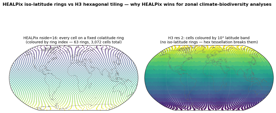
Wrapping up
Three HEALPix-family properties surveyed in this notebook:
Sphere ↔ ellipsoid mismatch (~0.7% systematic area bias at boreal latitudes) is negligible for biodiversity counts in isolation but material for the Copernicus × Destination Earth integration regime that ESA GRID4EARTH targets. Solutions:
rhealpixdggs(PyPI) or “Ellipsoidal HEALPix” via authalic-sphere mapping (GRID4EARTH).NESTED bit-shift refinement makes zoom-in / zoom-out O(1) per cell. No projection, no resampling, no hash lookup. Critical for Copernicus Zarr × biodiversity tile pipelines.
Iso-latitude pixelization makes zonal climate-zone analyses essentially free — group pixels by ring, no spatial query needed.
Together with the count-bias arguments (notebooks 01–02, 07) and the shape-preservation arguments (notebooks 03–04), these are why HEALPix is the right substrate for the integrated future where biodiversity, high-resolution Copernicus EO, and Destination Earth climate-model output share one common DGGS — not because HEALPix is uniquely best for biodiversity counts in isolation, but because the climate-model and spherical-ML sides already live on it and integration cost dominates. For biodiversity-only work at coarse resolution, any of the equal-area DGGS in notebook 07 works fine.