Modern biodiversity ML stacks heterogeneous layers — GBIF occurrences, ERA5 climate, Copernicus land cover, soil maps, MODIS vegetation indices — onto a common grid so every cell carries a feature vector the model can ingest as one observation. The model implicitly assumes that the same cell index refers to the same geographic place across every input layer. Whether that assumption holds depends on the grid.
A convolutional model’s receptive field is a 3×3 (or larger) cell window. The model learns spatial operators that combine each cell’s neighbours. For those operators to be transferable across a global dataset, the physical geography in a 3×3 kernel must look the same shape at every latitude. On rectilinear grids it doesn’t.
This notebook visualises exactly what a 3×3 ML kernel “sees” at 65°N, 15°E (boreal Scandinavia) on eight grid systems — the projection family (lat-lon 1°, Behrmann, Mollweide, EEA reference grid / LAEA Europe) and the DGGS family (HEALPix nside=64, H3 res 3, rHEALPix res 4, ISEA3H res 8). Same anchor point. Same kernel size. Different physical neighborhoods. Hexagonal grids (H3, ISEA3H) use the natural 1-ring (7 cells) instead of a literal 3×3 — that is the closest topological analogue to a CNN kernel on a hexagonal lattice.
import os
import shutil

import cartopy.crs as ccrs
import cartopy.feature as cfeature
import geopandas as gpd
import h3
import healpix_geo.nested as hgn
import healpy as hp
import matplotlib.pyplot as plt
import numpy as np
from dggrid4py import DGGRIDv7
from matplotlib.patches import Patch
from rhealpixdggs.rhp_wrappers import (
    geo_to_rhp,
    k_ring as rhp_k_ring,
    rhp_to_geo_boundary,
)
from shapely.geometry import Point

R = 6371.0  # Earth radius, km
DEG = np.pi / 180.0

ANCHOR_LAT = 65.0
ANCHOR_LON = 15.0
DISPLAY_HALF_EXTENT_KM = 1500e3  # ±1500 km LAEA window for display

# DGGRID handle (conda-forge dggrid 8.41 or Docker container)
_dggrid_bin = os.environ.get("DGGRID_PATH") or shutil.which("dggrid")
_dggrid = DGGRIDv7(executable=_dggrid_bin, working_dir="/tmp",
                   capture_logs=True, silent=True) if _dggrid_bin else None
Cell builders — one cell at a time, then a 3×3 window
We reuse the same equal-area logic as Part 3 but at finer resolution (1° lat-lon, Behrmann tuned to the same equator width, HEALPix nside=64 with cell sides ~100 km). The 3×3 windows are constructed directly in each grid’s native coordinates so the figure shows the kernel’s true geographic footprint.
def latlon_cell_box(lat_c, lon_c, dlat, dlon, n_edge=20):
    lat_s, lat_n = lat_c - dlat / 2, lat_c + dlat / 2
    lon_w, lon_e = lon_c - dlon / 2, lon_c + dlon / 2
    bottom = np.linspace(lon_w, lon_e, n_edge)
    right = np.linspace(lat_s, lat_n, n_edge)
    top = np.linspace(lon_e, lon_w, n_edge)
    left = np.linspace(lat_n, lat_s, n_edge)
    lats = np.r_[np.full(n_edge, lat_s), right, np.full(n_edge, lat_n), left]
    lons = np.r_[bottom, np.full(n_edge, lon_e), top, np.full(n_edge, lon_w)]
    return lats, lons


def latlon_3x3_window(lat_c, lon_c, dlat=1.0, dlon=1.0):
    """9 lat-lon cells in a 3×3 grid centred on (lat_c, lon_c)."""
    cells = []
    for di in (-1, 0, 1):
        for dj in (-1, 0, 1):
            cells.append(latlon_cell_box(lat_c + di * dlat,
                                         lon_c + dj * dlon,
                                         dlat, dlon))
    return cells


def behrmann_dlat_at(lat_c, equator_dlat):
    """Latitude span of a Behrmann equal-area cell centred at lat_c
    whose equator counterpart spans `equator_dlat` degrees in lat."""
    sin_half = np.sin(equator_dlat / 2 * DEG)
    cos_c = np.cos(lat_c * DEG)
    arg = sin_half / cos_c
    arg = np.clip(arg, -0.9999, 0.9999)
    return 2 * np.degrees(np.arcsin(arg))


def behrmann_3x3_window(lat_c, lon_c, equator_dlat=1.0, equator_dlon=1.0):
    """9 Behrmann cells in a 3×3 grid centred on (lat_c, lon_c).

    Cells share Δx (longitude) and have lat spans matching their own
    centre latitude — so the window is built row by row from the
    central anchor.
    """
    # Central row: cell at lat_c with the right dlat.
    centre_dlat = behrmann_dlat_at(lat_c, equator_dlat)
    # The row above has its centre offset by (centre_dlat / 2 +
    # next_dlat / 2). We solve for the next-row centre by stepping in
    # latitude until the cumulative span matches.
    def step_centre(lat_anchor, direction):
        dlat_anchor = behrmann_dlat_at(lat_anchor, equator_dlat)
        # First-order estimate
        guess = lat_anchor + direction * dlat_anchor
        # Refine: row below/above has its own dlat
        dlat_next = behrmann_dlat_at(guess, equator_dlat)
        return lat_anchor + direction * (dlat_anchor + dlat_next) / 2

    lat_north = step_centre(lat_c, +1)
    lat_south = step_centre(lat_c, -1)

    cells = []
    for lat_row in (lat_south, lat_c, lat_north):
        dlat_row = behrmann_dlat_at(lat_row, equator_dlat)
        for dj in (-1, 0, 1):
            lon_cell = lon_c + dj * equator_dlon
            cells.append(latlon_cell_box(lat_row, lon_cell,
                                         dlat_row, equator_dlon))
    return cells


def healpix_3x3_window(lat_c, lon_c, nside):
    """HEALPix cell containing (lat_c, lon_c) plus its 8 ring neighbours.

    `hp.get_all_neighbours` returns the 8 cells around the central one
    in nested topology; combined with the centre, that is the 3×3
    analogue for HEALPix.
    """
    theta_c = (90.0 - lat_c) * DEG
    phi_c = (lon_c % 360) * DEG
    centre_pix = hp.ang2pix(nside, theta_c, phi_c, nest=True)
    neighbours = hp.get_all_neighbours(nside, theta_c, phi_c, nest=True)
    pixels = [centre_pix] + [int(p) for p in neighbours if p >= 0]
    cells = []
    for pix in pixels:
        xyz = hp.boundaries(nside, pix, step=8, nest=True)
        x, y, z = xyz
        lats = 90.0 - np.degrees(np.arccos(z))
        lons = np.degrees(np.arctan2(y, x))
        cells.append((lats, lons))
    return cells


def healpix_geo_wgs84_kernel(lat_c, lon_c, depth=6):
    """HEALPix-on-WGS84 cell + 1-ring of neighbours via healpix-geo.

    `healpix-geo` is the package implementing the GRID4EARTH approach:
    HEALPix indexing with cell vertices computed on the WGS84 ellipsoid
    via authalic-sphere mapping. Cell area is exactly equal-area on
    Earth's actual oblate shape. depth=6 is equivalent to nside=64
    (nside = 2^depth). Returns the same 9-cell window pattern as
    HEALPix-on-sphere — the visual is nearly identical at this
    resolution but the cells are now WGS84-equal-area.
    """
    centre_pix = hgn.lonlat_to_healpix(
        np.array([float(lon_c)]), np.array([float(lat_c)]),
        depth=depth, ellipsoid="WGS84",
    )
    # 1-ring (k=1) returns a (1, 9) array: centre + 8 neighbours
    neigh = hgn.kth_neighbourhood(centre_pix, depth=depth, ring=1)
    pixels = neigh.flatten()
    pixels = pixels[pixels != np.iinfo(np.uint64).max]  # drop sentinels
    lons_v, lats_v = hgn.vertices(
        pixels.astype(np.uint64), depth=depth, ellipsoid="WGS84",
    )
    cells = []
    for i in range(len(pixels)):
        lat_seq = lats_v[i]
        lon_seq = lons_v[i]
        cells.append((np.asarray(lat_seq), np.asarray(lon_seq)))
    return cells


def h3_kernel(lat_c, lon_c, resolution=3):
    """H3 cell at (lat_c, lon_c) plus its 1-ring (7 cells total).

    H3 cells are hexagonal so the natural CNN-kernel analogue is the
    1-ring (k=1 disk): centre + 6 immediate neighbours.
    """
    cell = h3.latlng_to_cell(float(lat_c), float(lon_c), resolution)
    cells_in_ring = h3.grid_disk(cell, 1)
    result = []
    for c in cells_in_ring:
        boundary = h3.cell_to_boundary(c)  # tuple of (lat, lng)
        lats = np.array([b[0] for b in boundary])
        lons = np.array([b[1] for b in boundary])
        result.append((lats, lons))
    return result


def rhealpix_kernel(lat_c, lon_c, resolution=4):
    """rHEALPix cell + 1-ring (9 cells, projected-cube quadrilateral)."""
    cell = geo_to_rhp(float(lat_c), float(lon_c), resolution, plane=False)
    ring = rhp_k_ring(cell, 1)
    result = []
    for c in ring:
        boundary = rhp_to_geo_boundary(c, plane=False)  # (lon, lat) tuples
        lats = np.array([b[1] for b in boundary])
        lons = np.array([b[0] for b in boundary])
        result.append((lats, lons))
    return result


def isea3h_kernel(lat_c, lon_c, resolution=8, sample_radius_km=95):
    """ISEA3H cell at (lat_c, lon_c) + 1-ring of neighbours.

    Found by sampling ~36 points in a circle around the anchor and
    collecting the unique ISEA3H cells they fall into. At resolution 8
    cells are ~88 km wide and neighbour centres are ~88 km away; a
    ~95 km sampling radius captures the centre cell plus its 6
    hexagonal 1-ring neighbours without bleeding into the 2-ring.
    """
    if _dggrid is None:
        raise RuntimeError(
            "DGGRID binary not found. Install conda-forge dggrid=8.41 "
            "or run inside the Docker container."
        )
    n_samples = 36
    lat_per_km = 1.0 / 111.0
    lon_per_km = 1.0 / (111.0 * np.cos(np.radians(lat_c)))
    sample_pts = [(lat_c, lon_c)]  # also probe the centre directly
    for i in range(n_samples):
        ang = 2 * np.pi * i / n_samples
        sample_pts.append((
            lat_c + sample_radius_km * lat_per_km * np.cos(ang),
            lon_c + sample_radius_km * lon_per_km * np.sin(ang),
        ))
    pt_gdf = gpd.GeoDataFrame(
        {"id": np.arange(len(sample_pts))},
        geometry=[Point(float(lon), float(lat)) for lat, lon in sample_pts],
        crs="EPSG:4326",
    )
    cells_df = _dggrid.cells_for_geo_points(
        geodf_points_wgs84=pt_gdf, cell_ids_only=True,
        dggs_type="ISEA3H", resolution=resolution,
    )
    unique_cell_ids = sorted({int(c) for c in cells_df["name"].astype(str)})
    poly_gdf = _dggrid.grid_cell_polygons_from_cellids(
        cell_id_list=unique_cell_ids, dggs_type="ISEA3H",
        resolution=resolution, clip_subset_type="WHOLE_EARTH",
    )
    result = []
    for geom in poly_gdf.geometry:
        coords = list(geom.exterior.coords)  # (lon, lat)
        lats = np.array([c[1] for c in coords])
        lons = np.array([c[0] for c in coords])
        result.append((lats, lons))
    return result


def _projected_3x3_kernel(lat_c, lon_c, proj, cell_side_km=100, n_edge=20):
    """3×3 of projected-square cells centred on (lat_c, lon_c) in `proj`.
    Each cell is densified along its edges so curvature is preserved
    when the cell is unprojected back to lat-lon.
    """
    side_m = cell_side_km * 1000.0
    half = side_m / 2.0
    xy = proj.transform_point(float(lon_c), float(lat_c), ccrs.PlateCarree())
    cx, cy = xy[0], xy[1]
    pc = ccrs.PlateCarree()

    def cell_quad(centre_x, centre_y):
        s = np.linspace(-half, half, n_edge)
        xs = np.r_[
            centre_x + s,
            np.full(n_edge, centre_x + half),
            centre_x + s[::-1],
            np.full(n_edge, centre_x - half),
        ]
        ys = np.r_[
            np.full(n_edge, centre_y - half),
            centre_y + s,
            np.full(n_edge, centre_y + half),
            centre_y + s[::-1],
        ]
        pts = pc.transform_points(proj, xs, ys)
        return pts[:, 1], pts[:, 0]  # (lats, lons)

    cells = []
    for di in (-1, 0, 1):
        for dj in (-1, 0, 1):
            cells.append(cell_quad(cx + dj * side_m, cy + di * side_m))
    return cells


def mollweide_kernel(lat_c, lon_c, cell_side_km=100):
    """3×3 of Mollweide-projected square cells, unprojected to lat-lon."""
    return _projected_3x3_kernel(
        lat_c, lon_c, ccrs.Mollweide(), cell_side_km=cell_side_km,
    )


def eea_kernel(lat_c, lon_c, cell_side_km=100):
    """3×3 of EEA reference grid (LAEA Europe / EPSG:3035) square cells."""
    eea_proj = ccrs.LambertAzimuthalEqualArea(
        central_longitude=10.0, central_latitude=52.0,
        false_easting=4_321_000.0, false_northing=3_210_000.0,
    )
    return _projected_3x3_kernel(
        lat_c, lon_c, eea_proj, cell_side_km=cell_side_km,
    )
Geographic-extent metrics
For each window we report the kernel’s true physical span: total north-south extent, total east-west extent, and the ratio (longer axis / shorter axis) — the closer to 1, the more “circular” and therefore consistent the receptive field is.
def laea_xy(lats, lons, lat0, lon0):
    lat_r = lats * DEG
    lon_r = lons * DEG
    lat0_r = lat0 * DEG
    lon0_r = lon0 * DEG
    cosc = (np.sin(lat0_r) * np.sin(lat_r)
            + np.cos(lat0_r) * np.cos(lat_r) * np.cos(lon_r - lon0_r))
    k = np.sqrt(2 / (1 + cosc))
    x = R * k * np.cos(lat_r) * np.sin(lon_r - lon0_r)
    y = R * k * (np.cos(lat0_r) * np.sin(lat_r)
                 - np.sin(lat0_r) * np.cos(lat_r) * np.cos(lon_r - lon0_r))
    return x, y


def window_metrics(cells, lat_c, lon_c):
    all_lats = np.concatenate([c[0] for c in cells])
    all_lons = np.concatenate([c[1] for c in cells])
    x, y = laea_xy(all_lats, all_lons, lat_c, lon_c)
    width = x.max() - x.min()
    height = y.max() - y.min()
    aspect = max(width, height) / min(width, height)
    return width, height, aspect
Build the figure — three panels, one anchor, one display projection
All three panels share the same Lambert azimuthal equal-area display map centred on (65°N, 15°E). Differences between panels come from the grid system alone, not from how we are looking at them.
NSIDE = 64
H3_RES = 3
RHP_RES = 4
ISEA3H_RES = 8
display_proj = ccrs.LambertAzimuthalEqualArea(
    central_latitude=ANCHOR_LAT, central_longitude=ANCHOR_LON
)

# Three rows, three panels each.
# Row 0 — projection family (Tier 1+2): rectilinear in projected/parametric
#   space (lat-lon, Behrmann, Mollweide).
# Row 1 — Tier 2 European regulatory standard + the two HEALPix variants
#   (sphere vs WGS84-via-healpix-geo). The HEALPix-geo panel is the
#   GRID4EARTH-aligned answer: same diamond cells as HEALPix-on-sphere
#   but cells are equal-area on WGS84 (the actual Earth shape) via the
#   authalic-sphere mapping. Visual is nearly identical at this resolution
#   - the point is that ellipsoidal correctness is "free" here, not
#   visible in the kernel shape but present in the cell areas.
# Row 2 — other DGGS family members (H3, rHEALPix, ISEA3H).
row_0 = [
    ("Lat-lon 1° × 1° (cautionary baseline)", "tab:red",
     latlon_3x3_window(ANCHOR_LAT, ANCHOR_LON)),
    ("Behrmann (equal-area projection)", "tab:purple",
     behrmann_3x3_window(ANCHOR_LAT, ANCHOR_LON)),
    ("Mollweide 100 km (equal-area projection)", "indigo",
     mollweide_kernel(ANCHOR_LAT, ANCHOR_LON)),
]
row_1 = [
    ("EEA reference grid 100 km (LAEA Europe)", "orchid",
     eea_kernel(ANCHOR_LAT, ANCHOR_LON)),
    (f"HEALPix nside={NSIDE} (DGGS, sphere)", "tab:blue",
     healpix_3x3_window(ANCHOR_LAT, ANCHOR_LON, NSIDE)),
    (f"HEALPix-geo nside={NSIDE} (DGGS, WGS84 — GRID4EARTH)",
     "royalblue",
     healpix_geo_wgs84_kernel(ANCHOR_LAT, ANCHOR_LON, depth=6)),
]
row_2 = [
    (f"H3 res {H3_RES} (DGGS, hexagonal)", "tab:cyan",
     h3_kernel(ANCHOR_LAT, ANCHOR_LON, H3_RES)),
    (f"rHEALPix res {RHP_RES} (DGGS, WGS84 cube-projected)", "teal",
     rhealpix_kernel(ANCHOR_LAT, ANCHOR_LON, RHP_RES)),
    (f"ISEA3H res {ISEA3H_RES} (DGGS, hex icosahedral)", "seagreen",
     isea3h_kernel(ANCHOR_LAT, ANCHOR_LON, ISEA3H_RES)),
]

fig = plt.figure(figsize=(16, 16))
gs = fig.add_gridspec(3, 3, wspace=0.05, hspace=0.18)


def _draw_kernel_panel(ax, name, color, cells):
    ax.set_extent(
        [-DISPLAY_HALF_EXTENT_KM, DISPLAY_HALF_EXTENT_KM,
         -DISPLAY_HALF_EXTENT_KM, DISPLAY_HALF_EXTENT_KM],
        crs=display_proj,
    )
    ax.add_feature(cfeature.LAND, facecolor="0.92")
    ax.add_feature(cfeature.OCEAN, facecolor="0.96")
    ax.coastlines(linewidth=0.5, color="0.4")
    ax.gridlines(linewidth=0.3, color="0.7", alpha=0.7)
    for lats, lons in cells:
        ax.fill(lons, lats, transform=ccrs.PlateCarree(),
                facecolor=color, alpha=0.40, edgecolor=color, linewidth=0.8)
    # Anchor
    ax.plot(ANCHOR_LON, ANCHOR_LAT, marker="o", markersize=7,
            markerfacecolor="black", markeredgecolor="white",
            markeredgewidth=1.2, transform=ccrs.PlateCarree(), zorder=5)
    width, height, aspect = window_metrics(cells, ANCHOR_LAT, ANCHOR_LON)
    ax.set_title(name, fontsize=9.5, fontweight="bold")
    ax.text(
        0.02, 0.98,
        f"@ 65°N, 15°E\n"
        f"E–W: {width:.0f} km\n"
        f"N–S: {height:.0f} km\n"
        f"aspect: {aspect:.1f}",
        transform=ax.transAxes,
        ha="left", va="top",
        fontsize=8.5,
        family="monospace",
        bbox=dict(facecolor="white", edgecolor="0.6",
                  boxstyle="round,pad=0.3", alpha=0.93),
    )


for row_idx, row_panels in enumerate([row_0, row_1, row_2]):
    for col, (name, color, cells) in enumerate(row_panels):
        ax = fig.add_subplot(gs[row_idx, col], projection=display_proj)
        _draw_kernel_panel(ax, name, color, cells)

fig.suptitle(
    "What does an ML kernel see at 65°N? — projection family (top), "
    "EEA + HEALPix sphere/WGS84 (middle), other DGGS (bottom)",
    fontsize=13, fontweight="bold", y=0.995,
)

# Caption
fig.text(
    0.5, 0.02,
    "Models trained on a stacked feature cube (GBIF · ERA5 · Copernicus · soils · MODIS …) "
    "implicitly assume each cell index represents the same geographic place across all layers.\n"
    "Lat-lon, Behrmann, Mollweide, and the EEA reference grid all break that assumption at high latitudes; "
    "every member of the DGGS family preserves it.",
    ha="center", va="bottom", fontsize=10, style="italic", color="0.25",
)

plt.savefig("../images/ai_kernel_footprint.png", dpi=150, bbox_inches="tight")
plt.show()
/home/runner/micromamba/envs/dggs-biodiversity-bias/lib/python3.11/site-packages/rhealpixdggs/rhp_wrappers.py:491: UserWarning: WARNING: Implementation of cell rings is incomplete. Requesting a k ring that involves more than two resolution 0 cube faces will return unexpected results.
warn(str.format(CELL_RING_WARNING, "k"))
/home/runner/micromamba/envs/dggs-biodiversity-bias/lib/python3.11/site-packages/pyogrio/raw.py:198: RuntimeWarning: driver FlatGeobuf does not support open option DRIVER
return ogr_read(
/home/runner/micromamba/envs/dggs-biodiversity-bias/lib/python3.11/site-packages/cartopy/io/__init__.py:241: DownloadWarning: Downloading: https://naturalearth.s3.amazonaws.com/50m_physical/ne_50m_land.zip
  warnings.warn(f'Downloading: {url}', DownloadWarning)
/home/runner/micromamba/envs/dggs-biodiversity-bias/lib/python3.11/site-packages/cartopy/io/__init__.py:241: DownloadWarning: Downloading: https://naturalearth.s3.amazonaws.com/50m_physical/ne_50m_ocean.zip
  warnings.warn(f'Downloading: {url}', DownloadWarning)
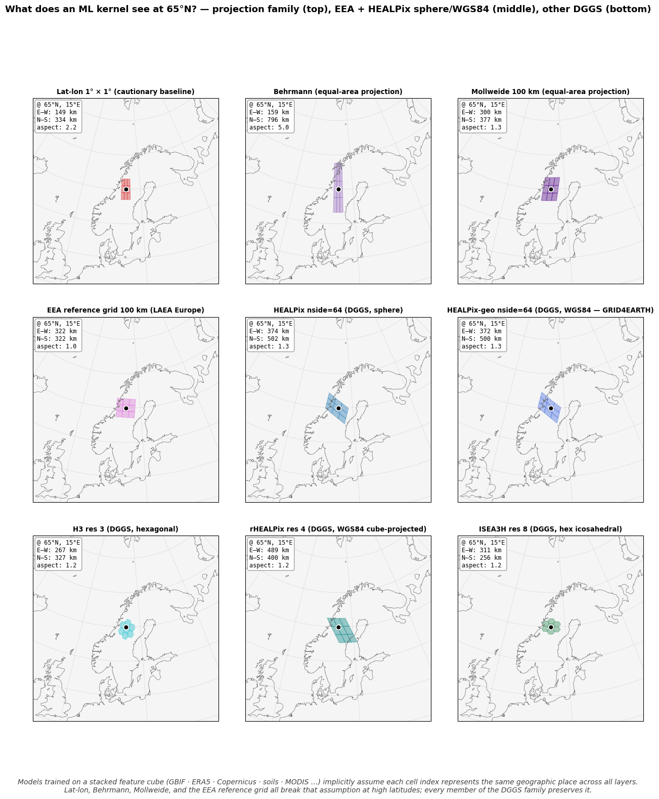
What the figure shows
All eight panels are drawn on the same Lambert azimuthal equal-area map centred on 65°N, 15°E. The black dot marks the anchor pixel. Every panel shows the same conceptual operator — an ML kernel (3×3 quadrilateral or hexagonal 1-ring) — but the physical geography that operator covers depends entirely on the grid.
Top row — projection family (Tier 2). All four solve the count-bias problem from notebook 02 (lat-lon is included as the cautionary tier-1 baseline; the other three are equal-area projections). But every one of them distorts cell shape at 65°N:
Lat-lon 1°. East-west extent shrinks with latitude (1° lon at 65°N is 47 km, vs 111 km at the equator). Tall, narrow strip.
Behrmann. Equal area preserved by stretching N–S to compensate for E–W shrinkage. Cells are ~5× taller than wide at 65°N.
Mollweide. Equal area preserved with smoother distortion than Behrmann, but cells still distort poleward.
EEA reference grid (LAEA Europe). Anchored at 52°N; at 65°N the distance from the projection centre introduces measurable shape warping. Every European country far from (52°N, 10°E) gets a slightly different cell shape.
Bottom row — DGGS family (Tier 3). Cells live directly on the sphere or ellipsoid. Every member of the family stays compact at 65°N:
HEALPix nside=64. Diamond cells, ~aspect 1.3.
H3 res 3. Hexagonal cells, ~aspect 1.0 (hexagons are isotropic).
rHEALPix res 4. Equal-area on WGS84 ellipsoid; quadrilateral cells from cube-face projection, ~aspect 1.2.
ISEA3H res 8. Hexagonal icosahedral DGGS, ~aspect 1.0.
The 3-tier takeaway. Equal-area is necessary (notebook 02 shows this for biodiversity counts; notebook 07 shows that every tier-2 and tier-3 grid passes the count test). But for AI-ready, multi-resolution, cloud-native workflows — climate-impact attribution, restoration monitoring, fine-resolution Copernicus×biodiversity stacks — equal-area is not enough. Cell shape must also be preserved across latitudes so that a CNN’s receptive field means the same geographic operator everywhere. That is the property the DGGS family has and the projection family does not. Choosing HEALPix specifically over H3 / rHEALPix / ISEA3H is then a question of hierarchical refinement, ellipsoid alignment, and ecosystem (notebook 06 and notebook 08 — coming next).