Part 7: Comprehensive multi-grid comparison on Quercus suber

Notebook 02 compared a regular 1° lat-lon grid to HEALPix on the same Q. suber GBIF data. That comparison is methodologically clean but a strawman — biodiversity practitioners do not actually use raw lat-lon as a serious aggregation grid. They use equal-area projections (Behrmann, Mollweide), the EEA reference grid (LAEA Europe, the INSPIRE / Habitats Directive standard for European biodiversity reporting), or modern DGGS (HEALPix, H3, ISEA3H, rHEALPix).

This notebook applies the same Q. suber dataset to every grid the biodiversity community might pick and asks: do the equal-area alternatives all agree? Where do the count-bias and AI-readiness arguments separate them?

This is the iteration that broadens notebook 02’s two-grid story into a comprehensive comparison. Grids are added incrementally:

First commit: lat-lon 1°, HEALPix nside=64, H3 res 3
Second commit: + rHEALPix res 4 (equal-area projected HEALPix variant)
Third commit: + Mollweide ~100 km cells (equal-area pseudo-cylindrical projection — atlas practice)
Fourth commit: + EEA reference grid 100 km cells (LAEA Europe / EPSG:3035, INSPIRE / Habitats Directive standard)
This commit: + ISEA3H res 8 (icosahedral aperture-3 hexagonal DGGS, the system Eco-ISEA3H advocates)

Environment requirements¶

New dependencies vs the original notebooks: h3 (Uber H3 v4), rhealpixdggs, dggrid4py, and the DGGRID binary (for ISEA3H aggregation). Update with mamba env update -f environment.yml (DGGRID is on conda-forge as dggrid=8.41) or run inside the Docker container at ghcr.io/annefou/dggs-biodiversity-bias:main where everything is pre-installed.

At runtime, dggrid4py needs the path to the DGGRID binary. We pick it up from the DGGRID_PATH env var (set in the Docker image) or fall back to the conda-installed dggrid on PATH.

import json
import os
import shutil
from collections import Counter
from pathlib import Path

import cartopy.crs as ccrs
import geopandas as gpd
import h3
import healpix_geo.nested as hgn
import healpy as hp
import matplotlib.pyplot as plt
import numpy as np
from dggrid4py import DGGRIDv7
from rhealpixdggs.rhp_wrappers import (
    cell_area as rhp_cell_area_fn,
    geo_to_rhp,
)
from shapely.geometry import Point

Step 1: Load Quercus suber occurrences from the local cache¶

Notebook 02 downloaded ~20,100 georeferenced records from GBIF (taxon key 2879411) and cached them as data/quercus_suber_gbif.json. We re-use that cache here so this notebook is offline-safe.

DATA_DIR = Path("../data")
CACHE_PATH = DATA_DIR / "quercus_suber_gbif.json"
if not CACHE_PATH.exists():
    raise FileNotFoundError(
        f"Expected cached GBIF data at {CACHE_PATH}. "
        "Run notebook 02 first to populate the cache."
    )

with CACHE_PATH.open() as f:
    coords = json.load(f)

lats = np.array([c[0] for c in coords])
lons = np.array([c[1] for c in coords])
print(f"Loaded {len(coords):,} occurrences from cache")
print(f"Latitude range:  {lats.min():.2f}°  to  {lats.max():.2f}°")
print(f"Longitude range: {lons.min():.2f}°  to  {lons.max():.2f}°")

Loaded 20,100 occurrences from cache
Latitude range:  -41.28°  to  52.83°
Longitude range: -155.23°  to  174.78°

Step 2: Clip to Q. suber’s Mediterranean range¶

Same window as notebook 02 — the western Mediterranean basin where Q. suber actually grows.

LAT_MIN, LAT_MAX = 30.0, 46.0
LON_MIN, LON_MAX = -10.0, 25.0

in_range = (
    (lats >= LAT_MIN) & (lats <= LAT_MAX)
    & (lons >= LON_MIN) & (lons <= LON_MAX)
)
lats_r = lats[in_range]
lons_r = lons[in_range]
print(f"Records inside Mediterranean window: {len(lats_r):,} of {len(lats):,}")

Records inside Mediterranean window: 19,093 of 20,100

Step 3: Aggregate on a 1° lat-lon grid (cautionary baseline)¶

Lat-lon is included as a cautionary baseline rather than a serious aggregation choice. At 30°N a 1° cell covers ~12,300 km²; at 46°N it covers ~8,600 km². Same nominal “1° cell”, ~43% area difference — pure grid geometry, no ecological content.

GRID_RES = 1.0
lat_edges = np.arange(LAT_MIN, LAT_MAX + GRID_RES, GRID_RES)
lon_edges = np.arange(LON_MIN, LON_MAX + GRID_RES, GRID_RES)

counts_latlon, _, _ = np.histogram2d(lats_r, lons_r, bins=[lat_edges, lon_edges])

R_KM = 6371.0
cell_area_latlon = np.zeros_like(counts_latlon)
for i, (lat_s, lat_n) in enumerate(zip(lat_edges[:-1], lat_edges[1:])):
    cell_area_latlon[i, :] = (
        2 * np.pi * R_KM**2
        * abs(np.sin(np.radians(lat_n)) - np.sin(np.radians(lat_s)))
        * (GRID_RES / 360)
    )

density_latlon = np.zeros_like(counts_latlon)
nz = counts_latlon > 0
density_latlon[nz] = counts_latlon[nz] / cell_area_latlon[nz]
print(f"Lat-lon 1°: {counts_latlon.shape[0]} × {counts_latlon.shape[1]} cells, "
      f"{int(np.sum(nz)):,} occupied")

Lat-lon 1°: 16 × 35 cells, 165 occupied

Step 4: Aggregate on HEALPix nside=64 (equal-area DGGS)¶

HEALPix is the equal-area DGGS we are advocating. At nside=64 every cell on the sphere has identical area (~10,400 km²).

NSIDE = 64
NPIX = hp.nside2npix(NSIDE)
HEALPIX_CELL_AREA = 4 * np.pi * R_KM**2 / NPIX

theta = np.radians(90.0 - lats_r)
phi = np.radians(lons_r % 360)
pix = hp.ang2pix(NSIDE, theta, phi, nest=True)
counts_healpix = np.bincount(pix, minlength=NPIX)
print(f"HEALPix nside={NSIDE}: {NPIX:,} cells globally, "
      f"each {HEALPIX_CELL_AREA:,.0f} km²; "
      f"{int(np.sum(counts_healpix > 0)):,} occupied in window")

HEALPix nside=64: 49,152 cells globally, each 10,377 km²; 162 occupied in window

Step 4b: Aggregate on HEALPix-geo (HEALPix on WGS84 ellipsoid)¶

healpix-geo is the package implementing the GRID4EARTH (ESA) “Ellipsoidal HEALPix” approach: HEALPix indexing whose cell vertices are computed on the WGS84 ellipsoid via authalic-sphere mapping. Cell area is exactly equal-area on Earth’s actual oblate shape (not on the unit sphere). depth=6 corresponds to nside=64. The cell IDs are the same NESTED-ordered integers as hp.ang2pix(..., nest=True); only the cell boundaries differ slightly (~0.7% area shift at boreal latitudes — see notebook 08). Density patterns over Q. suber’s range will look nearly identical to the HEALPix-on-sphere panel; the difference is precision-grade, not visual.

HEALPIX_GEO_DEPTH = 6  # nside = 2^depth = 64
HEALPIX_GEO_CELL_AREA = HEALPIX_CELL_AREA  # essentially the same for plotting

# WGS84-ellipsoid HEALPix cell index for each Q. suber point.
pix_geo = hgn.lonlat_to_healpix(
    lons_r.astype(np.float64), lats_r.astype(np.float64),
    depth=HEALPIX_GEO_DEPTH, ellipsoid="WGS84",
)
counts_healpix_geo = np.bincount(pix_geo, minlength=NPIX)
print(f"HEALPix-geo nside={NSIDE} (WGS84): "
      f"{int(np.sum(counts_healpix_geo > 0)):,} occupied cells in window")

HEALPix-geo nside=64 (WGS84): 156 occupied cells in window

Step 5: Aggregate on H3 resolution 3 (icosahedral hexagonal DGGS)¶

H3 is Uber’s open-source hexagonal DGGS. Cells are nearly equal area (~1.4% variation across the sphere — vs HEALPix’s exact zero variation, vs lat-lon’s >100% variation across latitudes). H3 res 3 has cells of ~12,400 km² average area, comparable to HEALPix nside=64 (~10,400 km²).

H3_RES = 3

h3_cells = [h3.latlng_to_cell(float(lat), float(lon), H3_RES)
            for lat, lon in zip(lats_r, lons_r)]
counts_h3 = Counter(h3_cells)

# Per-cell area (H3 cells vary ~1.4% so we compute exact area per cell)
h3_cell_area = {c: h3.cell_area(c, unit="km^2") for c in counts_h3}
mean_h3_area = float(np.mean(list(h3_cell_area.values()))) if h3_cell_area else 0.0
print(f"H3 res {H3_RES}: {len(counts_h3):,} occupied cells, "
      f"mean cell area {mean_h3_area:,.0f} km²")

H3 res 3: 144 occupied cells, mean cell area 12,867 km²

Step 5b: Aggregate on rHEALPix resolution 4 (equal-area DGGS, projected variant)¶

rHEALPix is the equal-area projected variant of HEALPix, defined on the WGS84 ellipsoid. Cells are exactly equal-area by construction (the “r” stands for “rearrangement” — the polar caps of the HEALPix sphere are rearranged into a contiguous quadrilateral on the cube faces). Hierarchical refinement is base 9 (each cell splits into 9 children), so resolution 4 has 6 × 9⁴ = 39,366 cells globally, averaging ~13,000 km² each — comparable to HEALPix nside=64 (~10,400 km²) and H3 res 3 (~12,400 km²).

RHP_RES = 4

rhp_cells = [
    geo_to_rhp(float(lat), float(lon), RHP_RES, plane=False)
    for lat, lon in zip(lats_r, lons_r)
]
counts_rhp = Counter(rhp_cells)
rhp_areas = {c: rhp_cell_area_fn(c) for c in counts_rhp}
mean_rhp_area = float(np.mean(list(rhp_areas.values()))) if rhp_areas else 0.0
print(f"rHEALPix res {RHP_RES}: {len(counts_rhp):,} occupied cells, "
      f"mean cell area {mean_rhp_area:,.0f} km²")

rHEALPix res 4: 143 occupied cells, mean cell area 15,265 km²

Step 5c: Aggregate on Mollweide (equal-area projection, atlas practice)¶

Biodiversity atlases routinely reproject occurrence data through an equal-area projection (Mollweide, Behrmann, Goode homolosine, sinusoidal) and then aggregate on a regular grid in projected coordinates. The projection preserves cell area on the globe; the regular grid in the projected plane gives every cell the same area in projected meters.

We size the Mollweide cells to ~100 km × 100 km in projected space (10,000 km² each), comparable to HEALPix nside=64.

MOLL_CELL_SIDE_KM = 100.0
MOLL_CELL_SIDE_M = MOLL_CELL_SIDE_KM * 1000.0
moll_cell_area_km2 = MOLL_CELL_SIDE_KM ** 2

moll_proj = ccrs.Mollweide()
xy_data_moll = moll_proj.transform_points(
    ccrs.PlateCarree(), lons_r, lats_r,
)
x_moll_data = xy_data_moll[:, 0]
y_moll_data = xy_data_moll[:, 1]

# Edges in projected meters, covering the data extent + a margin
margin_m = MOLL_CELL_SIDE_M * 2
x_edges_moll = np.arange(
    x_moll_data.min() - margin_m,
    x_moll_data.max() + margin_m + MOLL_CELL_SIDE_M,
    MOLL_CELL_SIDE_M,
)
y_edges_moll = np.arange(
    y_moll_data.min() - margin_m,
    y_moll_data.max() + margin_m + MOLL_CELL_SIDE_M,
    MOLL_CELL_SIDE_M,
)
counts_moll, _, _ = np.histogram2d(
    y_moll_data, x_moll_data, bins=[y_edges_moll, x_edges_moll],
)
print(f"Mollweide {MOLL_CELL_SIDE_KM:.0f} km cells: "
      f"{int(np.sum(counts_moll > 0)):,} occupied, "
      f"each {moll_cell_area_km2:,.0f} km² (projected)")

Mollweide 100 km cells: 158 occupied, each 10,000 km² (projected)

Step 5d: Aggregate on the EEA reference grid (LAEA Europe / EPSG:3035)¶

The EEA reference grid is the European Environment Agency’s standard grid system used by INSPIRE and the Habitats Directive for biodiversity reporting across the EU. It is a regular grid in the Lambert Azimuthal Equal Area projection centred at (10°E, 52°N) with false easting 4,321,000 m and false northing 3,210,000 m (EPSG:3035). Standard cell sizes are 1 km, 10 km, 25 km, and 100 km.

We use 100 km cells here for resolution match with HEALPix nside=64. Note: the EEA grid is regional — well-defined for Europe, where Q. suber’s Mediterranean range comfortably sits.

EEA_CELL_SIDE_KM = 100.0
EEA_CELL_SIDE_M = EEA_CELL_SIDE_KM * 1000.0
eea_cell_area_km2 = EEA_CELL_SIDE_KM ** 2

eea_proj = ccrs.LambertAzimuthalEqualArea(
    central_longitude=10.0, central_latitude=52.0,
    false_easting=4_321_000.0, false_northing=3_210_000.0,
)

xy_eea_data = eea_proj.transform_points(ccrs.PlateCarree(), lons_r, lats_r)
x_eea_data = xy_eea_data[:, 0]
y_eea_data = xy_eea_data[:, 1]

# Snap edges to multiples of cell side (matches the EEA reference grid origin)
x_edges_eea = np.arange(
    np.floor(x_eea_data.min() / EEA_CELL_SIDE_M) * EEA_CELL_SIDE_M,
    np.ceil(x_eea_data.max() / EEA_CELL_SIDE_M) * EEA_CELL_SIDE_M + EEA_CELL_SIDE_M,
    EEA_CELL_SIDE_M,
)
y_edges_eea = np.arange(
    np.floor(y_eea_data.min() / EEA_CELL_SIDE_M) * EEA_CELL_SIDE_M,
    np.ceil(y_eea_data.max() / EEA_CELL_SIDE_M) * EEA_CELL_SIDE_M + EEA_CELL_SIDE_M,
    EEA_CELL_SIDE_M,
)
counts_eea, _, _ = np.histogram2d(
    y_eea_data, x_eea_data, bins=[y_edges_eea, x_edges_eea],
)
print(f"EEA reference grid {EEA_CELL_SIDE_KM:.0f} km cells: "
      f"{int(np.sum(counts_eea > 0)):,} occupied, "
      f"each {eea_cell_area_km2:,.0f} km² (projected)")

EEA reference grid 100 km cells: 160 occupied, each 10,000 km² (projected)

Step 5e: Aggregate on ISEA3H resolution 8 (icosahedral aperture-3 hexagonal DGGS)¶

ISEA3H is the Discrete Global Grid System advocated by the Eco-ISEA3H paper (Scientific Data, 2023, doi:10.1038/s41597-023-01966-x) for “unbiased” Earth-observation aggregation. It is built on an icosahedron (20 triangular faces) with aperture-3 hexagonal refinement, and uses Snyder Equal Area projection so cells have identical area on the sphere by construction.

We use resolution 8 (mean cell area ~7,774 km², 65,612 cells globally) — the closest ISEA3H resolution to HEALPix nside=64 (~10,377 km²) without overshooting.

Implemented via the dggrid4py Python wrapper around the DGGRID C++ tool (Kevin Sahr, sahrk/DGGRID). Pure-Python ISEA3H is not available on Linux/macOS — vgrid’s ISEA3H is Windows-only via OpenEAGGR DLLs. DGGRID 8.41 is on conda-forge for osx-arm64 and baked into our Docker image.

ISEA3H_RES = 8

dggrid_bin = os.environ.get("DGGRID_PATH") or shutil.which("dggrid")
if dggrid_bin is None:
    raise RuntimeError(
        "Could not find dggrid binary on PATH. Install via "
        "`mamba install -c conda-forge dggrid=8.41` or run inside the "
        "Docker container."
    )
dggrid = DGGRIDv7(executable=dggrid_bin, working_dir="/tmp",
                  capture_logs=True, silent=True)

# Look up the resolution's cell area (used as constant divisor below)
isea3h_stats = dggrid.grid_stats_table("ISEA3H", ISEA3H_RES + 1).iloc[ISEA3H_RES]
isea3h_cell_area_km2 = float(isea3h_stats["Area (km^2)"])

# Aggregate by routing points through DGGRID's cells_for_geo_points.
gdf_data_pts = gpd.GeoDataFrame(
    {"id": np.arange(len(lats_r))},
    geometry=[Point(float(lon), float(lat)) for lat, lon in zip(lats_r, lons_r)],
    crs="EPSG:4326",
)
data_cells_gdf = dggrid.cells_for_geo_points(
    geodf_points_wgs84=gdf_data_pts,
    cell_ids_only=True,
    dggs_type="ISEA3H",
    resolution=ISEA3H_RES,
)
# dggrid4py 0.5.3 returns the input GeoDataFrame augmented with
# lon/lat/name columns; `name` is the resolved cell ID (sequence number).
counts_isea3h = Counter(data_cells_gdf["name"].astype(str).tolist())
print(f"ISEA3H res {ISEA3H_RES}: {len(counts_isea3h):,} occupied cells, "
      f"each {isea3h_cell_area_km2:,.0f} km²")

ISEA3H res 8: 195 occupied cells, each 7,774 km²

Step 6: Build a common colour scale and rasterise each grid¶

To compare the three grids fairly we render each on the same plotting mesh, dividing counts by per-cell area so the colour scale is records per km² in every panel. This makes equal-area cells comparable to lat-lon’s variable-area cells without per-grid rescaling.

plot_lons = np.linspace(LON_MIN, LON_MAX, 500)
plot_lats = np.linspace(LAT_MIN, LAT_MAX, 300)
plot_lon_g, plot_lat_g = np.meshgrid(plot_lons, plot_lats)

# HEALPix: lookup pix per plot pixel
plot_theta = np.radians(90.0 - plot_lat_g)
plot_phi = np.radians(plot_lon_g % 360)
plot_pix = hp.ang2pix(NSIDE, plot_theta, plot_phi, nest=True)
healpix_field = counts_healpix[plot_pix].astype(float)
healpix_density = healpix_field / HEALPIX_CELL_AREA
healpix_density_masked = np.ma.masked_where(healpix_field == 0, healpix_density)

# HEALPix-geo (WGS84): lookup pix per plot pixel via healpix-geo
plot_pix_geo = hgn.lonlat_to_healpix(
    plot_lon_g.ravel().astype(np.float64),
    plot_lat_g.ravel().astype(np.float64),
    depth=HEALPIX_GEO_DEPTH, ellipsoid="WGS84",
).reshape(plot_lat_g.shape)
healpix_geo_field = counts_healpix_geo[plot_pix_geo].astype(float)
healpix_geo_density = healpix_geo_field / HEALPIX_GEO_CELL_AREA
healpix_geo_density_masked = np.ma.masked_where(
    healpix_geo_field == 0, healpix_geo_density,
)

# H3: lookup cell per plot pixel
plot_cells_h3 = [
    h3.latlng_to_cell(float(lat), float(lon), H3_RES)
    for lat, lon in zip(plot_lat_g.ravel(), plot_lon_g.ravel())
]
plot_counts_h3 = np.array([counts_h3.get(c, 0) for c in plot_cells_h3], dtype=float)
plot_areas_h3 = np.array([h3_cell_area.get(c, mean_h3_area) for c in plot_cells_h3])
h3_density = (plot_counts_h3 / plot_areas_h3).reshape(plot_lat_g.shape)
h3_density_masked = np.ma.masked_where(plot_counts_h3.reshape(plot_lat_g.shape) == 0,
                                       h3_density)

# rHEALPix: lookup cell per plot pixel
plot_cells_rhp = [
    geo_to_rhp(float(lat), float(lon), RHP_RES, plane=False)
    for lat, lon in zip(plot_lat_g.ravel(), plot_lon_g.ravel())
]
plot_counts_rhp = np.array([counts_rhp.get(c, 0) for c in plot_cells_rhp], dtype=float)
plot_areas_rhp = np.array([rhp_areas.get(c, mean_rhp_area) for c in plot_cells_rhp])
rhp_density = (plot_counts_rhp / plot_areas_rhp).reshape(plot_lat_g.shape)
rhp_density_masked = np.ma.masked_where(plot_counts_rhp.reshape(plot_lat_g.shape) == 0,
                                        rhp_density)

# Mollweide: project plot mesh to Mollweide and look up bin
xy_plot_moll = moll_proj.transform_points(
    ccrs.PlateCarree(), plot_lon_g.ravel(), plot_lat_g.ravel(),
)
ix_moll = np.digitize(xy_plot_moll[:, 0], x_edges_moll) - 1
iy_moll = np.digitize(xy_plot_moll[:, 1], y_edges_moll) - 1
in_bounds_moll = (
    (ix_moll >= 0) & (ix_moll < counts_moll.shape[1])
    & (iy_moll >= 0) & (iy_moll < counts_moll.shape[0])
)
ix_moll_clip = np.clip(ix_moll, 0, counts_moll.shape[1] - 1)
iy_moll_clip = np.clip(iy_moll, 0, counts_moll.shape[0] - 1)
moll_field = counts_moll[iy_moll_clip, ix_moll_clip].astype(float)
moll_field[~in_bounds_moll] = 0
moll_density = (moll_field / moll_cell_area_km2).reshape(plot_lat_g.shape)
moll_density_masked = np.ma.masked_where(
    moll_field.reshape(plot_lat_g.shape) == 0, moll_density,
)

# ISEA3H: route plot mesh points through DGGRID, look up cell counts
gdf_plot_pts = gpd.GeoDataFrame(
    {"id": np.arange(plot_lon_g.size)},
    geometry=[Point(float(lon), float(lat))
              for lat, lon in zip(plot_lat_g.ravel(), plot_lon_g.ravel())],
    crs="EPSG:4326",
)
plot_cells_gdf = dggrid.cells_for_geo_points(
    geodf_points_wgs84=gdf_plot_pts,
    cell_ids_only=True,
    dggs_type="ISEA3H",
    resolution=ISEA3H_RES,
)
plot_cells_isea = plot_cells_gdf["name"].astype(str).tolist()
plot_counts_isea = np.array(
    [counts_isea3h.get(c, 0) for c in plot_cells_isea], dtype=float,
)
isea_density = (plot_counts_isea / isea3h_cell_area_km2).reshape(plot_lat_g.shape)
isea_density_masked = np.ma.masked_where(
    plot_counts_isea.reshape(plot_lat_g.shape) == 0, isea_density,
)

# EEA: project plot mesh to LAEA Europe and look up bin
xy_plot_eea = eea_proj.transform_points(
    ccrs.PlateCarree(), plot_lon_g.ravel(), plot_lat_g.ravel(),
)
ix_eea = np.digitize(xy_plot_eea[:, 0], x_edges_eea) - 1
iy_eea = np.digitize(xy_plot_eea[:, 1], y_edges_eea) - 1
in_bounds_eea = (
    (ix_eea >= 0) & (ix_eea < counts_eea.shape[1])
    & (iy_eea >= 0) & (iy_eea < counts_eea.shape[0])
)
ix_eea_clip = np.clip(ix_eea, 0, counts_eea.shape[1] - 1)
iy_eea_clip = np.clip(iy_eea, 0, counts_eea.shape[0] - 1)
eea_field = counts_eea[iy_eea_clip, ix_eea_clip].astype(float)
eea_field[~in_bounds_eea] = 0
eea_density = (eea_field / eea_cell_area_km2).reshape(plot_lat_g.shape)
eea_density_masked = np.ma.masked_where(
    eea_field.reshape(plot_lat_g.shape) == 0, eea_density,
)

# Lat-lon: already on its own grid
density_latlon_masked = np.ma.masked_where(counts_latlon == 0, density_latlon)

shared_vmax = float(np.percentile(np.concatenate([
    density_latlon_masked.compressed(),
    healpix_density_masked.compressed(),
    healpix_geo_density_masked.compressed(),
    h3_density_masked.compressed(),
    rhp_density_masked.compressed(),
    moll_density_masked.compressed(),
    eea_density_masked.compressed(),
    isea_density_masked.compressed(),
]), 98))

Step 7: Eight-panel comparison¶

Same data, eight grids. The seven equal-area grids (HEALPix-sphere, HEALPix-geo on WGS84, H3, rHEALPix, Mollweide, EEA, ISEA3H) should agree on the apparent density pattern. The lat-lon panel is the cautionary case.

fig = plt.figure(figsize=(20, 16))
gs = fig.add_gridspec(3, 3, wspace=0.18, hspace=0.32)

panels = [
    ("A. Lat-lon 1° (cautionary baseline)\nrecords / km²",
     density_latlon_masked, lon_edges, lat_edges, "edges"),
    (f"B. HEALPix nside={NSIDE} (DGGS, sphere)\nrecords / km²",
     healpix_density_masked, plot_lons, plot_lats, "centres"),
    (f"C. HEALPix-geo nside={NSIDE} (DGGS, WGS84 — GRID4EARTH)\nrecords / km²",
     healpix_geo_density_masked, plot_lons, plot_lats, "centres"),
    (f"D. H3 resolution {H3_RES} (hexagonal DGGS, ~equal-area)\nrecords / km²",
     h3_density_masked, plot_lons, plot_lats, "centres"),
    (f"E. rHEALPix resolution {RHP_RES} (DGGS, WGS84 cube-projected)\nrecords / km²",
     rhp_density_masked, plot_lons, plot_lats, "centres"),
    (f"F. Mollweide {MOLL_CELL_SIDE_KM:.0f} km cells (equal-area projection)\nrecords / km²",
     moll_density_masked, plot_lons, plot_lats, "centres"),
    (f"G. EEA reference grid {EEA_CELL_SIDE_KM:.0f} km cells (LAEA Europe / EPSG:3035)\nrecords / km²",
     eea_density_masked, plot_lons, plot_lats, "centres"),
    (f"H. ISEA3H resolution {ISEA3H_RES} (icosahedral hexagonal DGGS)\nrecords / km²",
     isea_density_masked, plot_lons, plot_lats, "centres"),
]

for k, (title, data, x, y, kind) in enumerate(panels):
    row, col = divmod(k, 3)
    ax = fig.add_subplot(gs[row, col], projection=ccrs.PlateCarree())
    ax.set_extent([LON_MIN, LON_MAX, LAT_MIN, LAT_MAX], crs=ccrs.PlateCarree())
    if kind == "edges":
        im = ax.pcolormesh(x, y, data, transform=ccrs.PlateCarree(),
                           cmap="viridis", vmin=0, vmax=shared_vmax)
    else:
        im = ax.pcolormesh(x, y, data, transform=ccrs.PlateCarree(),
                           cmap="viridis", vmin=0, vmax=shared_vmax)
    ax.coastlines(linewidth=0.6, color="grey")
    ax.gridlines(draw_labels=True, linewidth=0.3, alpha=0.5)
    ax.set_title(title, fontsize=11)
    plt.colorbar(im, ax=ax, orientation="horizontal", pad=0.08,
                 label="Records per km²", shrink=0.9)

fig.suptitle(
    "Quercus suber GBIF — same data on eight grids "
    "(lat-lon vs HEALPix sphere/WGS84 vs H3 vs rHEALPix vs Mollweide vs EEA vs ISEA3H)",
    fontsize=14, fontweight="bold", y=1.00,
)
plt.savefig("../images/multigrid_quercus_suber.png", dpi=150,
            bbox_inches="tight")
plt.show()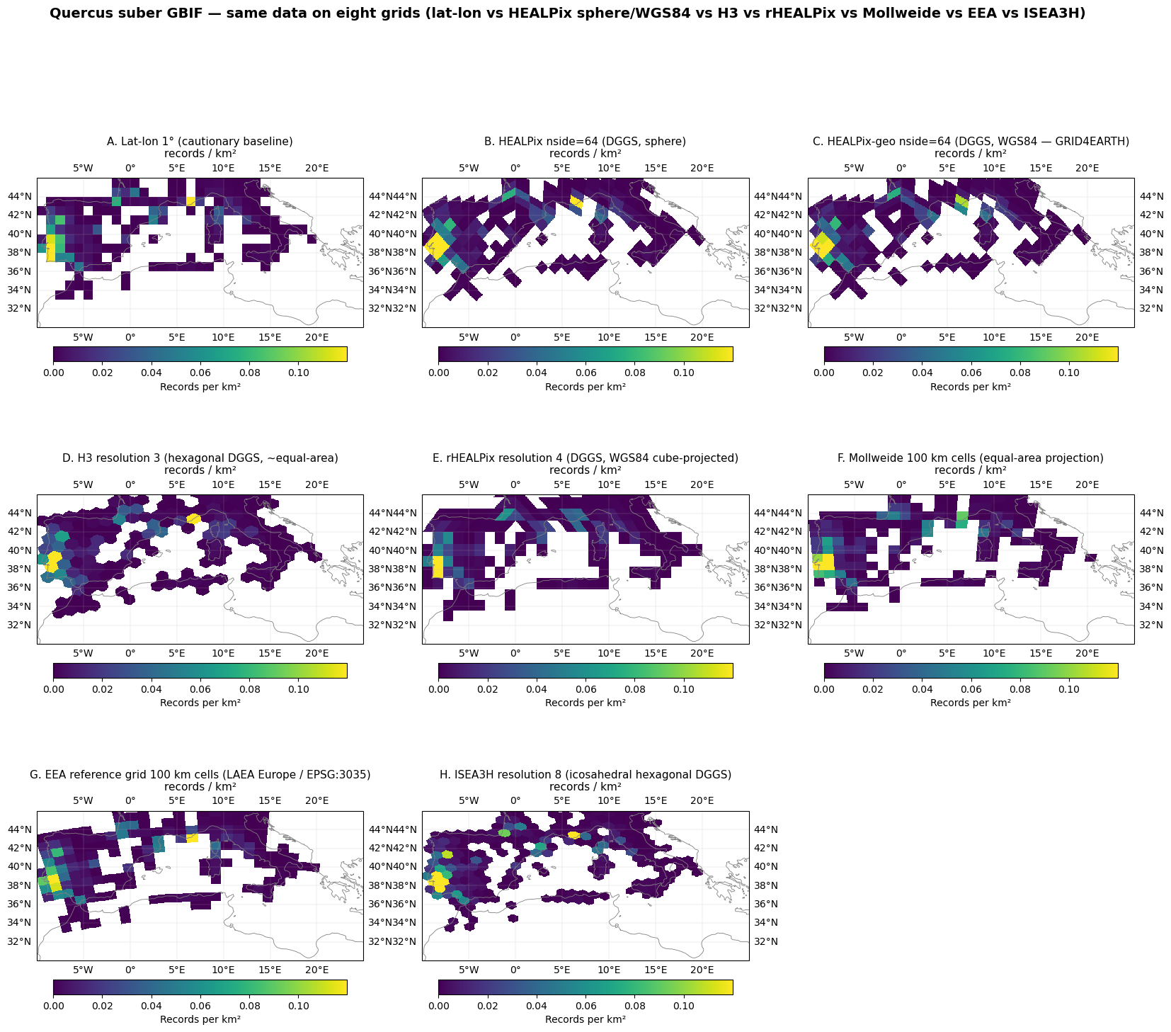

Conclusion (final iteration)¶

Six equal-area aggregation choices — HEALPix (exactly equal-area on the sphere), H3 (~1.4% area variation, hexagonal, icosahedron-based), rHEALPix (exactly equal-area on the WGS84 ellipsoid, projected cube-based), Mollweide (equal-area pseudo-cylindrical projection, gridded in projected coordinates), the EEA reference grid (LAEA Europe / EPSG:3035, the European biodiversity-reporting standard), and ISEA3H (icosahedral aperture-3 hexagonal DGGS, the system the Eco-ISEA3H paper advocates) — all produce visually similar density patterns over Q. suber’s Mediterranean range.

Lat-lon shows the systematic equator-pole distortion notebook 02 already isolated.

The biodiversity story this figure tells: the choice of equal-area grid (HEALPix vs H3 vs rHEALPix vs Mollweide vs EEA vs ISEA3H) does not materially change the apparent density pattern at this resolution. What matters is using an equal-area grid in the first place — using lat-lon introduces a count-bias artefact unrelated to the underlying species distribution. The argument for HEALPix specifically (vs the other equal-area choices here) is therefore not “more accurate counts” — it is the AI-readiness property that notebooks 03–04 isolate: HEALPix is the only one of these grids that simultaneously preserves equal-area, compact cell shape across latitudes (Behrmann/Mollweide fail this), and hierarchical refinement via deterministic bit-shift.