Part 2: Real GBIF data — Quercus suber (cork oak)

Part 1 proved with synthetic uniform data that a regular lat-lon grid produces systematic count bias even when the underlying density is constant. That was a mathematical property of the grid geometry.

This notebook asks the next question: does the same artefact show up in real biodiversity data? We use Quercus suber (cork oak), which is endemic to the western Mediterranean basin (~30–45°N) and is referenced in the EGU 2026 talk as a worked example.

Important caveat¶

Real occurrence data combines three signals:

Ecology — the species’ actual range and abundance.
Sampling effort — where biologists, citizen scientists, and institutions record observations.
Grid geometry — the cell-area artefact Part 1 isolated.

We cannot fully separate (1) and (2) from real data. What we can do, and what this notebook does, is quantify the (3) component directly: given the latitudinal range Q. suber actually occupies, how much of the variation in raw counts per lat-lon cell is explained by cell area alone?

import json
from pathlib import Path

import cartopy.crs as ccrs
import healpy as hp
import matplotlib.pyplot as plt
import numpy as np
import requests

Step 1: Download Quercus suber occurrences from GBIF¶

GBIF (https://www.gbif.org) is the global biodiversity data aggregator. We query the occurrence search API for georeferenced Q. suber records, filtering out those with known geospatial issues.

The notebook is self-contained: data is cached to ../data/ so subsequent runs skip the download.

GBIF_TAXON_KEY = 2879411  # Quercus suber
TARGET_RECORDS = 20_000   # search API hard-limits offset+limit at 100,000
PAGE_SIZE = 300

DATA_DIR = Path("../data")
DATA_DIR.mkdir(exist_ok=True)
CACHE_PATH = DATA_DIR / "quercus_suber_gbif.json"

USER_AGENT = (
    "dggs-biodiversity-bias/0.1 "
    "(EGU 2026 talk; https://github.com/sciencelivehub) "
    "python-requests"
)


def fetch_gbif_occurrences(taxon_key: int, target: int, page_size: int):
    coords = []
    offset = 0
    headers = {"User-Agent": USER_AGENT}
    while offset < target:
        r = requests.get(
            "https://api.gbif.org/v1/occurrence/search",
            params={
                "taxonKey": taxon_key,
                "hasCoordinate": "true",
                "hasGeospatialIssue": "false",
                "limit": page_size,
                "offset": offset,
            },
            headers=headers,
            timeout=60,
        )
        r.raise_for_status()
        payload = r.json()
        results = payload.get("results", [])
        if not results:
            break
        for rec in results:
            lat = rec.get("decimalLatitude")
            lon = rec.get("decimalLongitude")
            if lat is not None and lon is not None:
                coords.append((lat, lon))
        offset += page_size
        if payload.get("endOfRecords"):
            break
    return coords


if CACHE_PATH.exists():
    with CACHE_PATH.open() as f:
        coords = json.load(f)
    print(f"Loaded cached data: {len(coords):,} occurrences from {CACHE_PATH}")
else:
    print(f"Downloading up to {TARGET_RECORDS:,} occurrences from GBIF...")
    coords = fetch_gbif_occurrences(GBIF_TAXON_KEY, TARGET_RECORDS, PAGE_SIZE)
    with CACHE_PATH.open("w") as f:
        json.dump(coords, f)
    print(f"Downloaded {len(coords):,} occurrences, cached to {CACHE_PATH}")

lats = np.array([c[0] for c in coords])
lons = np.array([c[1] for c in coords])

print(f"Latitude range:  {lats.min():.2f}°  to  {lats.max():.2f}°")
print(f"Longitude range: {lons.min():.2f}°  to  {lons.max():.2f}°")

Loaded cached data: 20,100 occurrences from ../data/quercus_suber_gbif.json
Latitude range:  -41.28°  to  52.83°
Longitude range: -155.23°  to  174.78°

Step 2: Define the analysis region¶

Q. suber’s range is the western Mediterranean. We clip the analysis to a rectangular bounding box that covers it cleanly: 30–46°N, 10°W–25°E. Cells outside this box would just be empty.

LAT_MIN, LAT_MAX = 30.0, 46.0
LON_MIN, LON_MAX = -10.0, 25.0

in_range = (
    (lats >= LAT_MIN) & (lats <= LAT_MAX)
    & (lons >= LON_MIN) & (lons <= LON_MAX)
)
lats_r = lats[in_range]
lons_r = lons[in_range]
print(f"Records inside Mediterranean window: {len(lats_r):,} of {len(lats):,}")

Records inside Mediterranean window: 19,093 of 20,100

Step 3: Bin on a 1° regular lat-lon grid¶

A 1° grid is a common biodiversity-mapping resolution. At 30°N a 1° cell spans roughly 12,300 km²; at 46°N it spans roughly 8,600 km². The cell at 30°N is about 43% larger than the cell at 46°N — same nominal “1 degree” cell, very different ground area.

GRID_RES = 1.0  # degrees
lat_edges = np.arange(LAT_MIN, LAT_MAX + GRID_RES, GRID_RES)
lon_edges = np.arange(LON_MIN, LON_MAX + GRID_RES, GRID_RES)
lat_centers = (lat_edges[:-1] + lat_edges[1:]) / 2
lon_centers = (lon_edges[:-1] + lon_edges[1:]) / 2

counts_regular, _, _ = np.histogram2d(lats_r, lons_r, bins=[lat_edges, lon_edges])

R = 6371  # Earth radius, km
cell_areas_km2 = np.zeros_like(counts_regular)
for i, (lat_s, lat_n) in enumerate(zip(lat_edges[:-1], lat_edges[1:])):
    area = (
        2 * np.pi * R**2
        * abs(np.sin(np.radians(lat_n)) - np.sin(np.radians(lat_s)))
        * (GRID_RES / 360)
    )
    cell_areas_km2[i, :] = area

print(f"Lat-lon grid: {counts_regular.shape[0]} x {counts_regular.shape[1]} cells")
print(f"Cell area at {LAT_MIN:.0f}°N: {cell_areas_km2[0, 0]:>8,.0f} km²")
print(f"Cell area at {LAT_MAX:.0f}°N: {cell_areas_km2[-1, 0]:>8,.0f} km²")
print(f"Within-range area variation: "
      f"{(cell_areas_km2[0, 0] / cell_areas_km2[-1, 0] - 1) * 100:.1f}% "
      f"(southern cells are larger)")

Lat-lon grid: 16 x 35 cells
Cell area at 30°N:   10,653 km²
Cell area at 46°N:    8,666 km²
Within-range area variation: 22.9% (southern cells are larger)

Step 4: Bin on a HEALPix DGGS grid¶

HEALPix at nside=64 has cells of ~3,100 km² each — a comparable resolution to a 1° lat-lon cell at 40°N (~9,500 km²) but, crucially, the area is identical for every cell on the sphere.

NSIDE = 64
NPIX = hp.nside2npix(NSIDE)

theta = np.radians(90.0 - lats_r)
phi = np.radians(lons_r % 360)
pix = hp.ang2pix(NSIDE, theta, phi, nest=True)
counts_healpix = np.bincount(pix, minlength=NPIX)

healpix_cell_area = 4 * np.pi * R**2 / NPIX
print(f"HEALPix grid: nside={NSIDE}, {NPIX:,} cells globally")
print(f"Cell area (every cell): {healpix_cell_area:,.0f} km²")
print(f"Cells in Mediterranean window with ≥1 record: "
      f"{int(np.sum(counts_healpix > 0)):,}")

HEALPix grid: nside=64, 49,152 cells globally
Cell area (every cell): 10,377 km²
Cells in Mediterranean window with ≥1 record: 162

Step 5: How much of the lat-lon count signal is pure geometry?¶

This is the quantitative version of the synthetic argument from Part 1. We compare two views of the same 1° lat-lon data:

Raw counts per cell — what most biodiversity maps display.
Density (counts per km²) — corrects for cell area.

The two would be identical if cells had equal area. They don’t. The discrepancy is the part of the “raw count” map that is purely grid geometry, with no ecological content.

density_regular = np.zeros_like(counts_regular)
nonzero = counts_regular > 0
density_regular[nonzero] = counts_regular[nonzero] / cell_areas_km2[nonzero]

# For occupied cells, compute the geometry inflation factor:
# the same density at the southernmost vs northernmost row scales
# raw counts by area_south / area_north.
mean_lat_per_row = lat_centers
area_per_row = cell_areas_km2[:, 0]
geom_inflation = area_per_row / area_per_row.min()  # relative to smallest cell

print("Geometry inflation by latitude (relative to the smallest cell):")
for lat_c, infl in zip(mean_lat_per_row[::4], geom_inflation[::4]):
    print(f"  {lat_c:5.1f}°N: ×{infl:.2f}")

Geometry inflation by latitude (relative to the smallest cell):
   30.5°N: ×1.23
   34.5°N: ×1.18
   38.5°N: ×1.12
   42.5°N: ×1.05

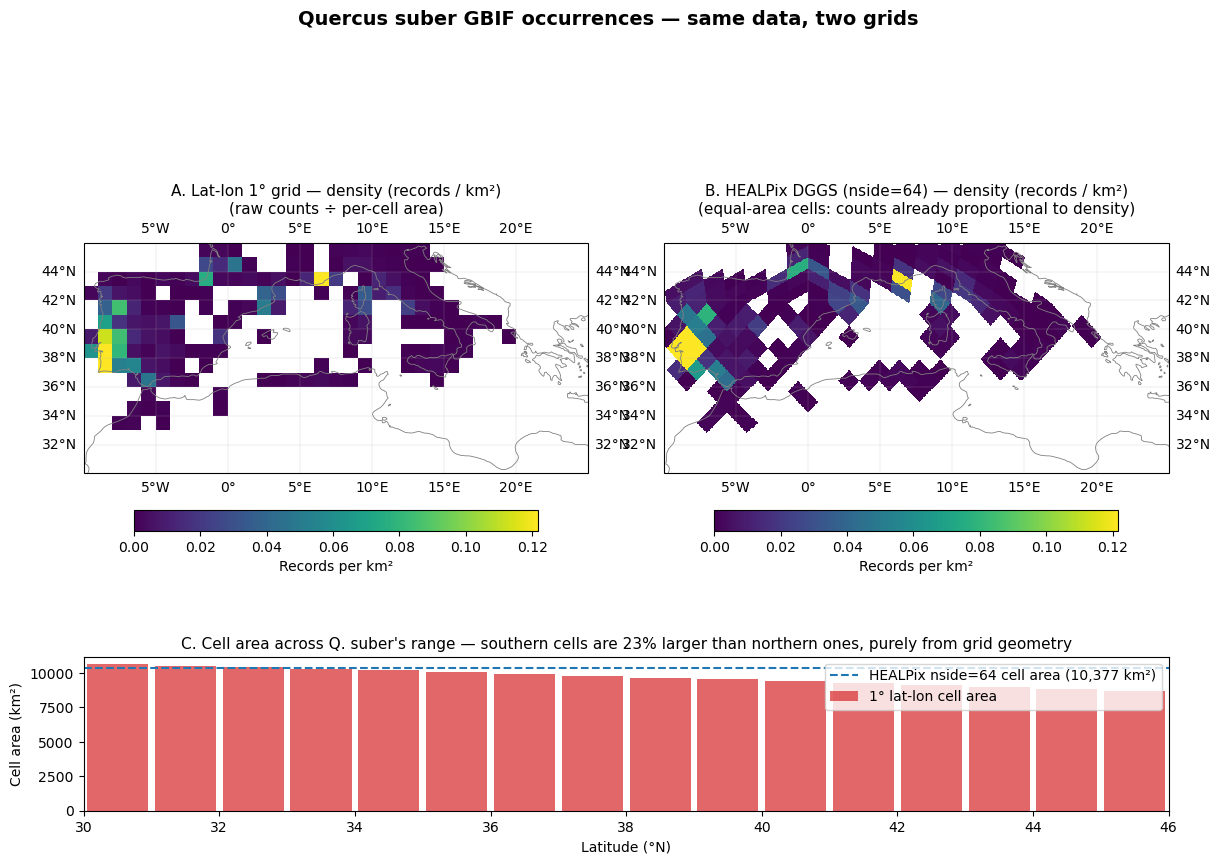
Step 6: The map — same data, two grids¶

The key visual: lat-lon raw counts vs HEALPix counts over Q. suber’s Mediterranean range. Both maps use the same colour scale, normalised by cell area so they are comparable in units of records per km² (i.e. density).

On the lat-lon map this normalisation is the per-cell area we just computed. On the HEALPix map every cell has the same area, so it is a single global divisor.

# Pre-compute everything we need so each panel is rendered exactly once.
density_lat_lon = np.ma.masked_where(counts_regular == 0, density_regular)

plot_lons = np.linspace(LON_MIN, LON_MAX, 500)
plot_lats = np.linspace(LAT_MIN, LAT_MAX, 300)
plot_lon_grid, plot_lat_grid = np.meshgrid(plot_lons, plot_lats)
plot_theta = np.radians(90.0 - plot_lat_grid)
plot_phi = np.radians(plot_lon_grid % 360)
plot_pix = hp.ang2pix(NSIDE, plot_theta, plot_phi, nest=True)
healpix_field = counts_healpix[plot_pix].astype(float)
healpix_masked = np.ma.masked_where(healpix_field == 0, healpix_field)
# Equal-area HEALPix counts already represent density up to a constant;
# divide by the (single) cell area so the colour bar reads records per km².
healpix_density_per_km2 = healpix_masked / healpix_cell_area

shared_vmax = float(
    np.percentile(np.concatenate([
        density_lat_lon.compressed(),
        healpix_density_per_km2.compressed(),
    ]), 98)
)

fig = plt.figure(figsize=(14, 9))
gs = fig.add_gridspec(2, 2, height_ratios=[3, 1], hspace=0.25, wspace=0.15)

# -- Panel A: lat-lon density (records / km²) ---------------------
ax_a = fig.add_subplot(gs[0, 0], projection=ccrs.PlateCarree())
ax_a.set_extent([LON_MIN, LON_MAX, LAT_MIN, LAT_MAX], crs=ccrs.PlateCarree())
im_a = ax_a.pcolormesh(
    lon_edges, lat_edges, density_lat_lon,
    transform=ccrs.PlateCarree(), cmap="viridis", vmin=0, vmax=shared_vmax,
)
ax_a.coastlines(linewidth=0.6, color="grey")
ax_a.gridlines(draw_labels=True, linewidth=0.3, alpha=0.5)
ax_a.set_title("A. Lat-lon 1° grid — density (records / km²)\n"
               "(raw counts ÷ per-cell area)", fontsize=11)
plt.colorbar(im_a, ax=ax_a, orientation="horizontal", pad=0.08,
             label="Records per km²", shrink=0.8)

# -- Panel B: HEALPix density (equal-area cells) ------------------
ax_b = fig.add_subplot(gs[0, 1], projection=ccrs.PlateCarree())
ax_b.set_extent([LON_MIN, LON_MAX, LAT_MIN, LAT_MAX], crs=ccrs.PlateCarree())
im_b = ax_b.pcolormesh(
    plot_lons, plot_lats, healpix_density_per_km2,
    transform=ccrs.PlateCarree(), cmap="viridis", vmin=0, vmax=shared_vmax,
)
ax_b.coastlines(linewidth=0.6, color="grey")
ax_b.gridlines(draw_labels=True, linewidth=0.3, alpha=0.5)
ax_b.set_title(f"B. HEALPix DGGS (nside={NSIDE}) — density (records / km²)\n"
               "(equal-area cells: counts already proportional to density)",
               fontsize=11)
plt.colorbar(im_b, ax=ax_b, orientation="horizontal", pad=0.08,
             label="Records per km²", shrink=0.8)

# -- Panel C: the geometry contribution ----------------------------
ax_c = fig.add_subplot(gs[1, :])
ax_c.bar(lat_centers, area_per_row, width=0.9, color="tab:red", alpha=0.7,
         label="1° lat-lon cell area")
ax_c.axhline(healpix_cell_area, color="tab:blue", linestyle="--",
             label=f"HEALPix nside={NSIDE} cell area "
                   f"({healpix_cell_area:,.0f} km²)")
ax_c.set_xlabel("Latitude (°N)")
ax_c.set_ylabel("Cell area (km²)")
ax_c.set_title(
    "C. Cell area across Q. suber's range — "
    f"southern cells are {(area_per_row.max()/area_per_row.min()-1)*100:.0f}% "
    "larger than northern ones, "
    "purely from grid geometry",
    fontsize=11,
)
ax_c.legend(loc="upper right")
ax_c.set_xlim(LAT_MIN, LAT_MAX)

fig.suptitle(
    "Quercus suber GBIF occurrences — same data, two grids",
    fontsize=14, fontweight="bold", y=1.00,
)
plt.savefig("../images/gbif_quercus_suber.png", dpi=150, bbox_inches="tight")
plt.show()

/home/runner/micromamba/envs/dggs-biodiversity-bias/lib/python3.11/site-packages/cartopy/io/__init__.py:241: DownloadWarning: Downloading: https://naturalearth.s3.amazonaws.com/50m_physical/ne_50m_coastline.zip
  warnings.warn(f'Downloading: {url}', DownloadWarning)

Conclusion¶

Within the cork oak’s actual range (~30–46°N), 1° lat-lon cells differ in area by tens of percent from south to north — purely from the geometry of the grid, with no ecological content. A “raw counts per cell” map therefore mixes three signals (real abundance, sampling effort, cell area) and inflates apparent abundance toward the equator. HEALPix removes the third signal entirely: every cell has identical area, so a count is a density up to a global constant.

This is the real-data analogue of the synthetic proof in Part 1. The mathematical artefact predicted there is present, measurable, and quantifiable in real GBIF data, even for a species with a narrow Mediterranean range. For analyses spanning broader latitudinal gradients (continental, hemispheric, global) the geometry contribution grows rapidly — at 60°N a 1° cell is half the area of one at the equator.

Equal-area is a statistical correctness choice, not a visualisation choice. Choosing HEALPix (or any equal-area DGGS) for biodiversity analysis makes counts and densities directly comparable across the globe without per-cell area corrections, and removes a source of bias that is invisible to the analyst but quantifiable to the geometer.