02 — Data clean: predictor layers on their native grids (Colombia window)

import json
import os
import zipfile
from pathlib import Path

import geopandas as gpd
import matplotlib.pyplot as plt
import numpy as np
import pandas as pd
import rasterio
import shapely
import xarray as xr
from osgeo import gdal
from rasterio.features import rasterize
from rasterio.transform import from_origin
from rasterio.windows import from_bounds
from scipy import ndimage, signal

gdal.UseExceptions()

RAW = Path("../data/raw")
SMOKE = os.environ.get("SMOKE", "0") == "1"
SMOKE_BBOX = (-75.0, 4.0, -73.0, 6.0)
CLEAN = Path("../data/clean_smoke" if SMOKE else "../data/clean")
FIGURES = Path("../figures/smoke" if SMOKE else "../figures")
CLEAN.mkdir(parents=True, exist_ok=True)
FIGURES.mkdir(parents=True, exist_ok=True)
SEED = 20261003

col = gpd.read_file(RAW / "gadm" / "gadm41_COL.gpkg", layer="ADM_ADM_0")
COL_GEOM = shapely.make_valid(col.geometry.iloc[0])
W, S, E, N = COL_GEOM.bounds
BBOX = (np.floor(W - 0.5), np.floor(S - 0.5), np.ceil(E + 0.5), np.ceil(N + 0.5))
print("window", BBOX)

WGS84_A, WGS84_F = 6378137.0, 1 / 298.257223563
E2 = WGS84_F * (2 - WGS84_F)


def metres_per_degree(lat: float) -> tuple[float, float]:
    """(north-south, east-west) metres per degree on the WGS84 ellipsoid at latitude lat."""
    phi = np.radians(lat)
    s2 = np.sin(phi) ** 2
    m = WGS84_A * (1 - E2) / (1 - E2 * s2) ** 1.5
    n = WGS84_A / np.sqrt(1 - E2 * s2)
    return float(np.radians(1) * m), float(np.radians(1) * n * np.cos(phi))


def grid_coords(transform, shape) -> tuple[np.ndarray, np.ndarray]:
    lon = transform.c + (np.arange(shape[1]) + 0.5) * transform.a
    lat = transform.f + (np.arange(shape[0]) + 0.5) * transform.e
    return lat, lon


def to_dataarray(arr: np.ndarray, transform, name: str, attrs: dict) -> xr.DataArray:
    lat, lon = grid_coords(transform, arr.shape)
    return xr.DataArray(arr, dims=("lat", "lon"), coords={"lat": lat, "lon": lon}, name=name, attrs=attrs)


def read_window(path: str, bbox=BBOX) -> tuple[np.ndarray, object, float | None]:
    with rasterio.open(path) as src:
        win = from_bounds(*bbox, transform=src.transform).round_offsets().round_lengths()
        return src.read(1, window=win, boundless=True, fill_value=src.nodata or 0), src.window_transform(win), src.nodata

WC_ZIP = (RAW / "worldclim" / "wc2.1_30s_bio.zip").resolve()
WC = [f"/vsizip/{WC_ZIP}/wc2.1_30s_bio_{i}.tif" for i in range(1, 20)]
SUPP_T1_SD = np.array([780.4, 362.0, 146.8, 103.1, 59.7])
pca_sample_path = CLEAN / "bioclim_pca_sample.parquet"

if SMOKE and not pca_sample_path.exists():
    rng = np.random.default_rng(SEED)
    lon = rng.uniform(SMOKE_BBOX[0], SMOKE_BBOX[2], 40_000)
    s0, s1 = np.sin(np.radians(SMOKE_BBOX[1])), np.sin(np.radians(SMOKE_BBOX[3]))
    lat = np.degrees(np.arcsin(rng.uniform(s0, s1, 40_000)))
    vals = {}
    for i, path in enumerate(WC, start=1):
        with rasterio.open(path) as src:
            win = from_bounds(*SMOKE_BBOX, transform=src.transform).round_offsets().round_lengths()
            a = src.read(1, window=win)
            wt = src.window_transform(win)
            r = np.clip(((wt.f - lat) / -wt.e).astype(int), 0, a.shape[0] - 1)
            c = np.clip(((lon - wt.c) / wt.a).astype(int), 0, a.shape[1] - 1)
            v = a[r, c].astype("float64")
            v[a[r, c] == src.nodata] = np.nan
            vals[f"bio{i}"] = v
            tr = src.transform
    sample = pd.DataFrame(vals)
    sample["row"] = ((tr.f - lat) / -tr.e).astype(int)
    sample["col"] = ((lon - tr.c) / tr.a).astype(int)
    sample = sample.dropna().iloc[:20_000]
    sample.to_parquet(pca_sample_path)
if not pca_sample_path.exists():
    rng = np.random.default_rng(SEED)
    with rasterio.open(WC[0]) as src:
        bio1 = src.read(1)
        tr, nod = src.transform, src.nodata
    rows_all, cols_all = [], []
    while sum(len(r) for r in rows_all) < 1_000_000:
        n = 3_000_000
        lon = rng.uniform(-180, 180, n)
        lat = np.degrees(np.arcsin(rng.uniform(-1, 1, n)))
        r = np.clip(((tr.f - lat) / -tr.e).astype(int), 0, bio1.shape[0] - 1)
        c = np.clip(((lon - tr.c) / tr.a).astype(int), 0, bio1.shape[1] - 1)
        ok = bio1[r, c] != nod
        rows_all.append(r[ok])
        cols_all.append(c[ok])
    rows = np.concatenate(rows_all)[:1_000_000]
    cols = np.concatenate(cols_all)[:1_000_000]
    del bio1
    vals = {}
    for i, path in enumerate(WC, start=1):
        with rasterio.open(path) as src:
            vals[f"bio{i}"] = src.read(1)[rows, cols].astype("float64")
        print("sampled", Path(path).name, flush=True)
    sample = pd.DataFrame(vals)
    sample["row"], sample["col"] = rows, cols
    sample.to_parquet(pca_sample_path)
sample = pd.read_parquet(pca_sample_path)
bio_cols = [f"bio{i}" for i in range(1, 20)]
X = sample[bio_cols].to_numpy()
print(len(X), "points; any NaN:", np.isnan(X).any())

pca_variants = {}
for name, scale in [("centre_only", False), ("centre_scale", True)]:
    mu = X.mean(axis=0)
    sd = X.std(axis=0, ddof=1) if scale else np.ones(X.shape[1])
    Z = (X - mu) / sd
    cov = np.cov(Z, rowvar=False)
    eigval, eigvec = np.linalg.eigh(cov)
    order = np.argsort(eigval)[::-1]
    eigval, eigvec = eigval[order], eigvec[:, order]
    pca_variants[name] = dict(center=mu, scale=sd, sdev=np.sqrt(eigval), rotation=eigvec,
                              prop=eigval / eigval.sum())
summary = pd.DataFrame({
    "component": [f"PC{i}" for i in range(1, 6)],
    "supp_table1_sd": SUPP_T1_SD,
    **{f"{k}_sd": v["sdev"][:5] for k, v in pca_variants.items()},
    **{f"{k}_cumprop": np.cumsum(v["prop"])[:5] for k, v in pca_variants.items()},
})
summary.to_csv(CLEAN / "bioclim_pca_summary.csv", index=False)
print(summary.to_string(index=False, float_format=lambda v: f"{v:.4g}"))
err = {k: float(np.abs(np.log(v["sdev"][:5] / SUPP_T1_SD)).mean()) for k, v in pca_variants.items()}
PCA_CHOICE = min(err, key=err.get)
print("mean |log SD ratio| vs Supp. Table 1:", err, "-> using", PCA_CHOICE)
pca = pca_variants[PCA_CHOICE]
pd.DataFrame(pca["rotation"][:, :5], index=bio_cols, columns=[f"PC{i}" for i in range(1, 6)]).assign(
    center=pca["center"], scale=pca["scale"]).to_csv(CLEAN / "bioclim_pca_loadings.csv")

pcs_out = CLEAN / "bioclim_pca.nc"
if not pcs_out.exists():
    stack = []
    for path in WC:
        arr, tr, nod = read_window(path)
        stack.append(np.where(arr == nod, np.nan, arr).astype("float64"))
    stack = np.stack(stack, axis=-1)
    Z = (stack - pca["center"]) / pca["scale"]
    pcs = Z @ pca["rotation"][:, :5]
    ds = xr.Dataset({f"pc{i + 1}": to_dataarray(pcs[..., i].astype("float32"), tr, f"pc{i + 1}", {})
                     for i in range(5)})
    ds.attrs = {"pca_variant": PCA_CHOICE, "source": "WorldClim v2.1 30 s bioclim; PCA on 1e6 global land points"}
    ds.to_netcdf(pcs_out)
print(xr.open_dataset(pcs_out))

CHELSA = ("https://os.zhdk.cloud.switch.ch/chelsav2/GLOBAL/climatologies/1981-2010/bio/"
          "CHELSA_bio{i}_1981-2010_V.2.1.tif")
chelsa_sample_path = CLEAN / "chelsa_pca_sample.parquet"
chelsa_win_path = CLEAN / "chelsa_window.nc"
gdal.SetConfigOption("GDAL_HTTP_MAX_RETRY", "10")
gdal.SetConfigOption("GDAL_HTTP_RETRY_DELAY", "5")
gdal.SetConfigOption("CPL_VSIL_CURL_CHUNK_SIZE", "8388608")
gdal.SetConfigOption("GDAL_DISABLE_READDIR_ON_OPEN", "EMPTY_DIR")

with rasterio.open(WC[0]) as src:
    wc_tr = src.transform
pt_lon = wc_tr.c + (sample["col"].to_numpy() + 0.5) * wc_tr.a
pt_lat = wc_tr.f + (sample["row"].to_numpy() + 0.5) * wc_tr.e

if not (chelsa_sample_path.exists() and chelsa_win_path.exists()):
    cvals, cwin = {}, {}
    for i in range(1, 20):
        with rasterio.open("/vsicurl/" + CHELSA.format(i=i)) as src:
            tr, sc, off = src.transform, src.scales[0], src.offsets[0]
            r = np.floor((tr.f - pt_lat) / -tr.e).astype(int)
            c = np.clip(np.floor((pt_lon - tr.c) / tr.a).astype(int), 0, src.width - 1)
            inside = (r >= 0) & (r < src.height)
            vals = np.full(len(pt_lon), np.nan)
            wwin = from_bounds(*BBOX, transform=tr).round_offsets().round_lengths()
            wr0, wr1 = int(wwin.row_off), int(wwin.row_off + wwin.height)
            win_rows = []
            step = 512
            for r0 in range(0, src.height, step):
                n = min(step, src.height - r0)
                need = inside & (r >= r0) & (r < r0 + n)
                touches_win = r0 < wr1 and r0 + n > wr0
                if not need.any() and not touches_win:
                    continue
                block = src.read(1, window=rasterio.windows.Window(0, r0, src.width, n))
                vals[need] = block[r[need] - r0, c[need]]
                if touches_win:
                    a, b = max(r0, wr0), min(r0 + n, wr1)
                    win_rows.append(block[a - r0:b - r0, int(wwin.col_off):int(wwin.col_off + wwin.width)])
            vals[vals == 65535] = np.nan
            cvals[f"bio{i}"] = vals * sc + off
            w = np.concatenate(win_rows).astype("float64")
            w[w == 65535] = np.nan
            cwin[f"bio{i}"] = (w * sc + off, src.window_transform(wwin))
        print("CHELSA bio", i, "done", flush=True)
    pd.DataFrame(cvals).to_parquet(chelsa_sample_path)
    wtr = cwin["bio1"][1]
    xr.Dataset({k: to_dataarray(v[0].astype("float32"), wtr, k, {}) for k, v in cwin.items()}).to_netcdf(chelsa_win_path)

csample = pd.read_parquet(chelsa_sample_path)
both_ok = ~csample[bio_cols].isna().any(axis=1).to_numpy()
print(f"CHELSA: {both_ok.sum():,} of {len(csample):,} sample points valid")
Xc = csample.loc[both_ok, bio_cols].to_numpy()
mu_c = Xc.mean(axis=0)
sd_c = Xc.std(axis=0, ddof=1) if PCA_CHOICE == "centre_scale" else np.ones(Xc.shape[1])
ev_c, evec_c = np.linalg.eigh(np.cov((Xc - mu_c) / sd_c, rowvar=False))
o = np.argsort(ev_c)[::-1]
ev_c, evec_c = ev_c[o], evec_c[:, o]
summary["chelsa_sd"] = np.sqrt(ev_c[:5])
summary["chelsa_cumprop"] = np.cumsum(ev_c / ev_c.sum())[:5]
summary.to_csv(CLEAN / "bioclim_pca_summary.csv", index=False)
print(summary.to_string(index=False, float_format=lambda v: f"{v:.4g}"))

cpcs_out = CLEAN / "chelsa_pca.nc"
if not cpcs_out.exists():
    cw = xr.open_dataset(chelsa_win_path)
    st = np.stack([cw[b].values.astype("float64") for b in bio_cols], axis=-1)
    cp = ((st - mu_c) / sd_c) @ evec_c[:, :5]
    lat, lon = cw.lat.values, cw.lon.values
    xr.Dataset({f"cpc{i + 1}": xr.DataArray(cp[..., i].astype("float32"), dims=("lat", "lon"),
                                            coords={"lat": lat, "lon": lon}) for i in range(5)},
               attrs={"pca_variant": PCA_CHOICE, "source": "CHELSA v2.1 1981-2010 bioclim; sensitivity check",
                      "url_template": CHELSA}).to_netcdf(cpcs_out)
print(xr.open_dataset(cpcs_out))

soil_out = CLEAN / "soil_0_30cm.nc"
if not soil_out.exists():
    layers = {}
    for var in ["OCDENS", "PHIHOX"]:
        xs = []
        for d in [1, 2, 3, 4]:
            with rasterio.open(RAW / "soilgrids2017" / f"{var}_M_sl{d}_colombia.tif") as src:
                a = src.read(1).astype("float32")
                nod = src.nodata
                tr = src.transform
            if nod is not None:
                a[a == nod] = np.nan
            xs.append(a)
        x1, x2, x3, x4 = xs
        layers[var.lower()] = to_dataarray(
            ((5 * (x1 + x2) / 2 + 10 * (x2 + x3) / 2 + 15 * (x3 + x4) / 2) / 30).astype("float32"), tr, var.lower(),
            {"units": "kg m-3" if var == "OCDENS" else "pH x 10", "depth": "0-30 cm trapezoidal"})
    xr.Dataset(layers).to_netcdf(soil_out)
print(xr.open_dataset(soil_out))

LC11 = {
    1: ("cropland", [10, 11, 12, 20]),
    2: ("mosaic cropland / natural vegetation", [30, 40]),
    3: ("tree cover", [50, 60, 61, 62, 70, 71, 72, 80, 81, 82, 90]),
    4: ("mosaic tree-shrub / herbaceous", [100, 110]),
    5: ("shrubland", [120, 121, 122]),
    6: ("grassland, lichens and mosses", [130, 140]),
    7: ("sparse vegetation", [150, 151, 152, 153]),
    8: ("flooded vegetation", [160, 170, 180]),
    9: ("urban", [190]),
    10: ("bare areas, permanent snow and ice", [200, 201, 202, 220]),
    11: ("water", [210]),
}
lut = np.zeros(256, dtype="uint8")
for k, (_, codes) in LC11.items():
    lut[codes] = k
pd.DataFrame([(k, v[0], " ".join(map(str, v[1]))) for k, v in LC11.items()],
             columns=["class", "name", "esa_cci_codes"]).to_csv(CLEAN / "landcover_classes.csv", index=False)

CROPLAND_CODES = [10, 11, 12, 20, 30]
CROP_RADIUS_M, LAT_REF = 5000.0, 0.5 * (S + N)


def disk_kernel(radius_m: float, dy_m: float, dx_m: float) -> np.ndarray:
    ry, rx = int(np.ceil(radius_m / dy_m)), int(np.ceil(radius_m / dx_m))
    yy, xx = np.mgrid[-ry:ry + 1, -rx:rx + 1]
    k = ((yy * dy_m) ** 2 + (xx * dx_m) ** 2 <= radius_m**2).astype("float32")
    return k / k.sum()


lc_out = CLEAN / "landcover.nc"
if not lc_out.exists():
    out = {}
    for year in [1992, 1999, 2000, 2015]:
        with rasterio.open(RAW / "esacci_lc" / f"esacci_lc_{year}_colombia.tif") as src:
            raw = src.read(1)
            tr = src.transform
        mdeg_y, mdeg_x = metres_per_degree(LAT_REF)
        dy, dx = abs(tr.e) * mdeg_y, tr.a * mdeg_x
        out[f"lc_{year}"] = to_dataarray(lut[raw], tr, f"lc_{year}", {"classes": "see landcover_classes.csv"})
        out[f"esa_{year}"] = to_dataarray(raw, tr, f"esa_{year}", {"legend": "ESA CCI LCCS"})
        if year in (2000, 2015):
            crop = np.isin(raw, CROPLAND_CODES).astype("float32")
            dens = signal.oaconvolve(crop, disk_kernel(CROP_RADIUS_M, dy, dx), mode="same")
            out[f"cropland_density_{year}"] = to_dataarray(np.clip(dens, 0, 1).astype("float32"), tr,
                                                           f"cropland_density_{year}", {"units": "fraction, 5 km radius"})
            urban = raw == 190
            dist = ndimage.distance_transform_edt(~urban, sampling=(dy, dx)).astype("float32")
            out[f"dist_urban_{year}"] = to_dataarray(dist, tr, f"dist_urban_{year}", {"units": "m"})
    xr.Dataset(out).to_netcdf(lc_out)
print(xr.open_dataset(lc_out))

npp_out = CLEAN / "npp.nc"
if not npp_out.exists():
    with rasterio.open(RAW / "npp" / "MOD17A3_NPP_mean_00_15_colombia.tif") as src:
        a = src.read(1).astype("float32")
        tr, nod = src.transform, src.nodata
    print("NPP raw range:", np.nanmin(a), np.nanmax(a), "nodata", nod)
    valid = (a >= 0) & (a <= 65500) & (a != (nod if nod is not None else -1))
    npp = np.where(valid, a * 0.0001, np.nan).astype("float32")  # kg C m-2 yr-1 (NTSG scale factor)
    xr.Dataset({"npp": to_dataarray(npp, tr, "npp", {"units": "kg C m-2 yr-1", "period": "mean 2000-2015"})}).to_netcdf(npp_out)
print(xr.open_dataset(npp_out))

roads_out = CLEAN / "roads.nc"
if not roads_out.exists():
    zpath = (RAW / "grip4" / "GRIP4_density_total.zip").resolve()
    tif = "grip4_total_dens_m_km2.asc"  # the zip also holds grip4_area_land_km2.asc (land area, not roads)
    assert tif in zipfile.ZipFile(zpath).namelist()
    a, tr, nod = read_window(f"/vsizip/{zpath}/{tif}")
    a = np.where(a == nod, np.nan, a).astype("float32") if nod is not None else a.astype("float32")
    xr.Dataset({"road_density": to_dataarray(a, tr, "road_density", {"units": "m km-2", "source": tif})}).to_netcdf(roads_out)
print(xr.open_dataset(roads_out))

burn_out = CLEAN / "burned.nc"
burned_source = json.load(open(RAW / ("burned_source_smoke.json" if SMOKE else "burned_source.json")))
print("burned-area source:", burned_source)
if not burn_out.exists() and burned_source["source"] != "globfire":
    if burned_source["source"] == "mcd64a1":
        with rasterio.open(RAW / "mcd64a1" / burned_source["mcd64a1_file"]) as src:
            cnt = src.read(1).astype("float32")
            tr = src.transform
        frac = cnt / burned_source["months"]
    else:
        res = 1 / 240
        tr = from_origin(BBOX[0], BBOX[3], res, res)
        frac = np.full((int(round((BBOX[3] - BBOX[1]) / res)), int(round((BBOX[2] - BBOX[0]) / res))), np.nan, "float32")
    xr.Dataset({"burned_frac": to_dataarray(frac.astype("float32"), tr, "burned_frac",
                                            {"units": "fraction of months burned", "source": burned_source["source"],
                                             "months": burned_source["months"]})}).to_netcdf(burn_out)
if not burn_out.exists():
    res = 1 / 240
    tr = from_origin(BBOX[0], BBOX[3], res, res)
    shape = (int(round((BBOX[3] - BBOX[1]) / res)), int(round((BBOX[2] - BBOX[0]) / res)))
    count = np.zeros(shape, dtype="uint16")
    BURN_TYPE = "FinalArea"  # final perimeter of each fire event (ActiveArea = daily spread)
    files = sorted((RAW / "globfire").glob("globfire_*_colombia.parquet"))
    if SMOKE:
        files = [f for f in files if f.name in ("globfire_2005_01_colombia.parquet", "globfire_2005_02_colombia.parquet")]
    else:
        files = [f for f in files if 2001 <= int(f.name.split("_")[1]) <= 2017]
    assert len(files) == burned_source["months"], (len(files), burned_source)
    types = {}
    for f in files:
        g = gpd.read_parquet(f)
        for t, n in g["Type"].value_counts().items():
            types[t] = types.get(t, 0) + n
        g = g[g["Type"] == BURN_TYPE]
        if len(g):
            count += rasterize(((geom, 1) for geom in g.geometry), out_shape=shape, transform=tr,
                               fill=0, dtype="uint8")
    print("GlobFire polygon types over all months:", types)
    frac = (count / len(files)).astype("float32")
    xr.Dataset({"burned_frac": to_dataarray(frac, tr, "burned_frac",
                                            {"units": "fraction of months burned", "months": len(files),
                                             "polygon_type": BURN_TYPE})}).to_netcdf(burn_out)
print(xr.open_dataset(burn_out))

biome_out = CLEAN / "biomes_colombia.parquet"
if not biome_out.exists():
    eco = gpd.read_file(f"/vsizip/{(RAW / 'ecoregions' / 'Ecoregions2017.zip').resolve()}", bbox=BBOX)
    eco = eco[["BIOME_NUM", "BIOME_NAME", "ECO_NAME", "geometry"]].copy()
    eco["geometry"] = shapely.make_valid(eco.geometry.values)
    biomes = eco.dissolve(by=["BIOME_NUM", "BIOME_NAME"], as_index=False)[["BIOME_NUM", "BIOME_NAME", "geometry"]]
    biomes["geometry"] = biomes.geometry.clip_by_rect(*BBOX)
    biomes.to_parquet(biome_out)
biomes = gpd.read_parquet(biome_out)
geod_areas = biomes.to_crs("EPSG:4326").geometry.intersection(COL_GEOM)
from pyproj import Geod  # noqa: E402

g = Geod(ellps="WGS84")
biomes["area_in_colombia_mha"] = [abs(g.geometry_area_perimeter(x)[0]) / 1e10 for x in geod_areas]
print(biomes.drop(columns="geometry").to_string(index=False))

for layer in ["treecover2000", "gain", "lossyear"]:
    files = sorted(str(p.resolve()) for p in (RAW / "hansen").glob(f"*_{layer}_*.tif"))
    gdal.BuildVRT(str(CLEAN / f"hansen_{layer}.vrt"), files).FlushCache()
srtm = sorted(f"/vsizip/{p.resolve()}/{p.name.replace('.SRTMGL1.hgt.zip', '.hgt')}"
              for p in (RAW / "srtm").glob("*.hgt.zip"))
gdal.BuildVRT(str(CLEAN / "srtm.vrt"), srtm).FlushCache()
for v in ["hansen_treecover2000.vrt", "srtm.vrt"]:
    with rasterio.open(CLEAN / v) as src:
        print(v, src.bounds, src.res, src.dtypes)

fig, axes = plt.subplots(1, 4, figsize=(16, 5))
pcs = xr.open_dataset(pcs_out)
soil = xr.open_dataset(soil_out)
lc = xr.open_dataset(lc_out)
for ax, (da, title) in zip(axes, [(pcs.pc1, "bioclim PC1"), (soil.ocdens, "OCDENS 0-30 cm"),
                                  (soil.phihox, "PHIHOX 0-30 cm"), (lc.lc_2000, "land cover 2000 (11 cl.)")]):
    da[::4, ::4].plot(ax=ax, add_colorbar=True)
    ax.set_title(title)
    ax.set_aspect("equal")
fig.tight_layout()
fig.savefig(FIGURES / "predictors_overview.png", dpi=150, bbox_inches="tight")
plt.show()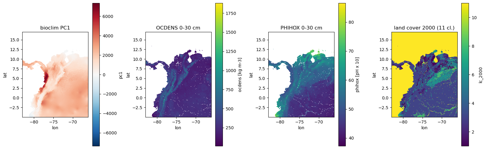

json.dump({"pca_variant": PCA_CHOICE, "pca_sd_error": err}, open(CLEAN / "clean_meta.json", "w"), indent=2)