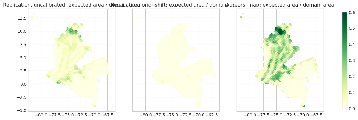
Our own implementation of the paper’s final spatial model (ten biophysical predictors), trained on Fagan et al. (2022) labels in Colombia, compared with the paper on accuracy and with the authors’ published map on area and spatial pattern.
Model. sklearn.ensemble.RandomForestClassifier set to R randomForest
classification defaults: 500 trees, mtry = floor(sqrt(10)) = 3
(max_features=3), nodesize = 1 (min_samples_leaf=1), bootstrap samples of
size n with replacement, Gini splits. Fully grown trees have pure leaves, so
predict_proba equals R’s vote fraction. Categorical predictors (land cover,
biome) are integer-coded (sklearn has no native categorical splits in random
forests; R does).
Sample size. Paper: final model on 1,000,000 balanced records, validation on 4.87 M independent balanced points. Scaled by Colombia’s share of the Fagan regrowth patches (188,921 / 4.78 M = 3.95 %): 39,523 training records. Validation uses every point in our independent validation set.
Areas. Exact WGS84 area of each 30 m pixel (primary); Mollweide (sphere
R = a) and nominal 0.09 ha as sensitivity columns. Areas are estimated from the
1-in-100 systematic grid of 02b (each grid pixel stands for 10 × 10 pixels).
Calibration (extension; the paper does not calibrate). The RF is trained on
50/50 samples, so its vote fractions are not probabilities at Colombia’s true
regrowth prevalence π. We report expected area (i) uncalibrated, as in the
paper, and (ii) after the prior-shift correction
p′ = π·p / (π·p + (1 − π)(1 − p)), with π = exact Fagan-regrowth area / exact
area of the sampling domain (class-0 ∪ class-1 masks, 30 m, from 02b). An
isotonic calibration fitted on one half of the validation set, weighted to
prevalence π, is a cross-check; the other half is used for evaluation
(Brier score, reliability diagram).
import json
import os
from pathlib import Path

import matplotlib.pyplot as plt
import numpy as np
import pandas as pd
import xarray as xr
from healpix_geo.nested import healpix_to_lonlat, lonlat_to_healpix
from scipy import stats
from sklearn.ensemble import RandomForestClassifier
from sklearn.isotonic import IsotonicRegression
from sklearn.metrics import brier_score_loss, cohen_kappa_score, confusion_matrix

plt.style.use("seaborn-v0_8-whitegrid")
SMOKE = os.environ.get("SMOKE", "0") == "1" # tiny test configuration (snakemake --config smoke=1)
CLEAN = Path("../data/clean_smoke" if SMOKE else "../data/clean")
RESULTS = Path("../results/smoke" if SMOKE else "../results")
FIGURES = Path("../figures/smoke" if SMOKE else "../figures")
DERIVED = Path("../data/derived_smoke" if SMOKE else "../data/derived")
STAGE_A = Path("../results") / "step1_authors_map_healpix_d8.nc"
N_TREES = 100 if SMOKE else 500
for d in (RESULTS, FIGURES, DERIVED):
d.mkdir(parents=True, exist_ok=True)
SEED = 20261003
MHA = 1e10
GRID_W = 100 # 10 x 10 pixels per systematic grid point
FINAL_VARS = ["forest_density_2000", "dist_forest_2000", "ocdens", "phihox", "pc1", "pc2", "pc3", "pc4", "lc_2000", "biome"]
PRED_MAP = {"forest_density_2000": "forest_density_2018", "dist_forest_2000": "dist_forest_2018", "lc_2000": "lc_2015"}
COL_SHARE = 188_921 / 4_780_000
N_TRAIN = 2_000 if SMOKE else int(round(1_000_000 * COL_SHARE))
PAPER = dict(val_acc=0.879, oob_acc=0.878, neotropics_oa=0.865, pnr_continuous_mha=11.19, pnr_binary_mha=13.70,
available_mha=93.78)
samples = pd.read_parquet(CLEAN / "samples.parquet")
grid = pd.read_parquet(CLEAN / "pred_grid.parquet")
sums = pd.read_csv(CLEAN / "tile_sums.csv").drop(columns="tile").sum()
meta = json.load(open(CLEAN / "features_meta.json"))
print(samples.groupby(["set", "label"]).size(), "\n", len(grid), "grid points;", meta)set label
train_pool 0 75990
1 75990
validation 0 61678
1 61678
dtype: int64
12161726 grid points; {'TREE_THRESHOLD': 30, 'DENSITY_RADIUS_M': 1000.0, 'DIST_CAP_M': 25000.0, 'GRID_STRIDE': 10, 'TARGET_PER_CLASS': 214809, 'RATE0': 0.0007049645526895149, 'RATE1': 0.09729694934810547, 'n_candidates': 455224, 'n_per_class': 137668, 'n_tiles': 121}
rng = np.random.default_rng(SEED)
pool = samples[samples.set == "train_pool"]
val = samples[samples.set == "validation"].reset_index(drop=True)
train = pd.concat([g.sample(n=min(N_TRAIN // 2, len(g)), random_state=SEED) for _, g in pool.groupby("label")])
print("training records:", len(train), train.label.value_counts().to_dict(), "| validation:", len(val))


def make_rf(max_features: int = 3, seed: int = SEED) -> RandomForestClassifier:
    return RandomForestClassifier(n_estimators=N_TREES, max_features=max_features, min_samples_leaf=1, bootstrap=True,
                                  oob_score=True, n_jobs=-1, random_state=seed)


rf = make_rf().fit(train[FINAL_VARS].to_numpy(), train.label.to_numpy())
p_val = rf.predict_proba(val[FINAL_VARS].to_numpy())[:, 1]
y_val = val.label.to_numpy()
val_acc = float(((p_val > 0.5) == y_val).mean())
cm = confusion_matrix(y_val, p_val > 0.5)
tn, fp, fn, tp = cm.ravel()
print(f"OOB accuracy {rf.oob_score_:.4f} (paper {PAPER['oob_acc']}); validation accuracy {val_acc:.4f} "
      f"(paper {PAPER['val_acc']})")
print(pd.DataFrame(cm, index=["ref 0", "ref 1"], columns=["map 0", "map 1"]))
imp = pd.Series(rf.feature_importances_, index=FINAL_VARS).sort_values(ascending=False)
print("Gini importance:\n", imp.round(4).to_string())
training records: 39522 {0: 19761, 1: 19761} | validation: 123356
OOB accuracy 0.8844 (paper 0.878); validation accuracy 0.8867 (paper 0.879)
       map 0  map 1
ref 0  56766   4912
ref 1   9066  52612
Gini importance:
 dist_forest_2000       0.2732
forest_density_2000    0.1927
phihox                 0.1142
pc2                    0.0853
pc1                    0.0780
pc3                    0.0749
pc4                    0.0743
ocdens                 0.0712
lc_2000                0.0287
biome                  0.0075
Prevalence and calibration
PI = float(sums["class1_area_ell"] / (sums["class1_area_ell"] + sums["class0_area_ell"]))
print(f"prevalence pi = {sums['class1_area_ell'] / 1e4:,.0f} ha regrowth / "
      f"{(sums['class1_area_ell'] + sums['class0_area_ell']) / MHA:.3f} Mha sampling domain = {PI:.5f}")


def prior_shift(p: np.ndarray, pi: float = PI, train_prev: float = 0.5) -> np.ndarray:
    num = p * pi / train_prev
    return num / (num + (1 - p) * (1 - pi) / (1 - train_prev))


half = rng.permutation(len(val)) < len(val) // 2  # True = calibration-fit half, False = evaluation half
w_val = np.where(y_val == 1, PI, 1 - PI) / np.where(y_val == 1, (y_val == 1).mean(), (y_val == 0).mean())
iso = IsotonicRegression(out_of_bounds="clip", y_min=0, y_max=1).fit(p_val[half], y_val[half], sample_weight=w_val[half])
ev = ~half
scores = {"uncalibrated": p_val[ev], "prior_shift": prior_shift(p_val[ev]), "isotonic": iso.predict(p_val[ev])}
brier = {k: float(brier_score_loss(y_val[ev], s, sample_weight=w_val[ev])) for k, s in scores.items()}
print("Brier score on the prevalence-weighted evaluation half:", brier)
prevalence pi = 251,707 ha regrowth / 15.307 Mha sampling domain = 0.01644
Brier score on the prevalence-weighted evaluation half: {'uncalibrated': 0.0708721991620386, 'prior_shift': 0.008147165560779194, 'isotonic': 0.00806318948344988}
bins = np.linspace(0, 1, 11)
fig, ax = plt.subplots(figsize=(5.5, 5))
rel_rows = []
for k, s in scores.items():
    idx = np.clip(np.digitize(s, bins) - 1, 0, 9)
    for b in range(10):
        sel = idx == b
        if w_val[ev][sel].sum() > 0:
            rel_rows.append(dict(score=k, bin=b, mean_pred=np.average(s[sel], weights=w_val[ev][sel]),
                                 obs_freq=np.average(y_val[ev][sel], weights=w_val[ev][sel]), n=int(sel.sum())))
rel = pd.DataFrame(rel_rows)
for k, g in rel.groupby("score"):
    ax.plot(g.mean_pred, g.obs_freq, "o-", label=f"{k} (Brier {brier[k]:.4f})")
ax.plot([0, 1], [0, 1], "k--", lw=0.8)
ax.set_xlabel("mean predicted probability")
ax.set_ylabel(f"observed regrowth frequency (weighted to prevalence {PI:.4f})")
ax.set_title("Step 2 reliability (validation half not used for fitting)")
ax.legend(fontsize=8)
fig.savefig(FIGURES / "step2_reliability.png", dpi=150, bbox_inches="tight")
plt.show()
rel.to_csv(RESULTS / "step2_reliability.csv", index=False)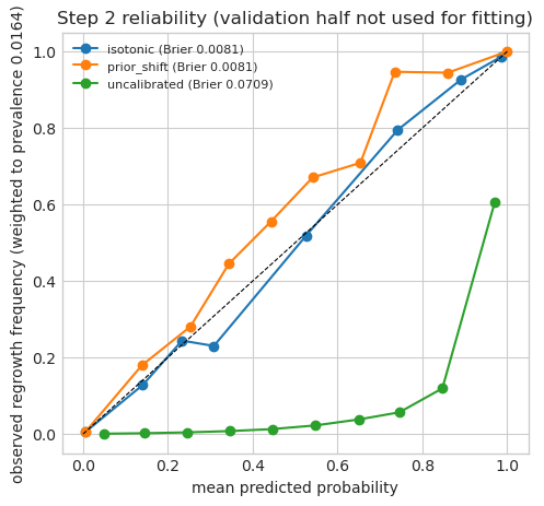
Prediction on the systematic grid and areas
g = grid[grid.is_pred_domain].copy()
Xp = g[[PRED_MAP.get(v, v) for v in FINAL_VARS]].to_numpy()
ok = ~np.isnan(Xp).any(axis=1)
print(f"prediction-domain grid points {len(g):,}; with complete predictors {ok.sum():,} ({ok.mean():.4%})")
g = g[ok].copy()
g["p"] = rf.predict_proba(Xp[ok])[:, 1]
g["p_prior"] = prior_shift(g.p.to_numpy())
g["p_iso"] = iso.predict(g.p.to_numpy())

A = 6378137.0


def sphere_over_ellipsoid(lat: np.ndarray) -> np.ndarray:
    res = 0.00025
    f = 1 / 298.257223563
    e2 = f * (2 - f)
    e = np.sqrt(e2)
    q = lambda phi: (1 - e2) * (np.sin(phi) / (1 - e2 * np.sin(phi) ** 2)  # noqa: E731
                                - np.log((1 - e * np.sin(phi)) / (1 + e * np.sin(phi))) / (2 * e))
    top, bot = np.radians(lat + res / 2), np.radians(lat - res / 2)
    return (A**2 * (np.sin(top) - np.sin(bot))) / (A**2 / 2 * (q(top) - q(bot)))


def area_estimates(df: pd.DataFrame, weight: np.ndarray) -> dict[str, float]:
    a_ell = df.area_ell.to_numpy() * GRID_W
    y = weight * a_ell
    n = len(y)
    se = np.sqrt(n * y.var(ddof=1) * (1 - 1 / GRID_W)) if n > 1 else np.nan  # SRS approximation, conservative
    return {"ell": y.sum() / MHA, "ell_se": se / MHA,
            "sph": (y * sphere_over_ellipsoid(df.lat.to_numpy())).sum() / MHA,
            "nom": (weight * 900.0 * GRID_W).sum() / MHA}


rows = []


def add(metric: str, est: dict | float, paper: float | None = None, note: str = "") -> None:
    if isinstance(est, dict):
        rows.append(dict(metric=metric, value=est["ell"], se=est.get("ell_se"), mollweide_sphere=est["sph"],
                         nominal_009ha=est["nom"], paper_value=paper, note=note))
    else:
        rows.append(dict(metric=metric, value=est, se=None, mollweide_sphere=None, nominal_009ha=None,
                         paper_value=paper, note=note))


add("oob_accuracy", float(rf.oob_score_), PAPER["oob_acc"])
add("validation_accuracy", val_acc, PAPER["val_acc"], f"n={len(val)} balanced; paper Neotropics OA 0.865")
add("validation_users_accuracy_regrowth", float(tp / (tp + fp)), 0.92, "paper SI A1.2 global")
add("validation_producers_accuracy_regrowth", float(tp / (tp + fn)), 0.852, "paper SI A1.2 global (count based)")
add("prevalence_pi", PI, None, "Fagan regrowth area / sampling-domain area, exact 30 m")
for k, v in brier.items():
    add(f"brier_{k}", v, None, "evaluation half of validation, weighted to prevalence")
add("expected_area_uncalibrated_mha", area_estimates(g, g.p.to_numpy()), PAPER["pnr_continuous_mha"],
    "sum p x area, as in the paper")
add("expected_area_prior_shift_mha", area_estimates(g, g.p_prior.to_numpy()), None, "calibrated to prevalence")
add("expected_area_isotonic_mha", area_estimates(g, g.p_iso.to_numpy()), None, "cross-check")
add("area_p_gt_0.5_uncalibrated_mha", area_estimates(g, (g.p > 0.5).to_numpy().astype(float)), PAPER["pnr_binary_mha"])
add("area_p_gt_0.5_prior_shift_mha", area_estimates(g, (g.p_prior > 0.5).to_numpy().astype(float)), None)
add("area_p_gt_0.5_isotonic_mha", area_estimates(g, (g.p_iso > 0.5).to_numpy().astype(float)), None)
add("prediction_domain_area_mha", {"ell": sums["pred_area_ell"] / MHA, "sph": sums["pred_area_sph"] / MHA,
                                   "nom": sums["pred_n"] * 900 / MHA}, PAPER["available_mha"], "exact 30 m count")
add("study_domain_area_mha", {"ell": sums["domain_area_ell"] / MHA, "sph": sums["domain_area_sph"] / MHA,
                              "nom": sums["domain_n"] * 900 / MHA}, PAPER["available_mha"], "Colombia x biomes 1-3")
for k, lab, paper in [("expected", "authors_expected", PAPER["pnr_continuous_mha"]),
                      ("bin1", "authors_binary", PAPER["pnr_binary_mha"]),
                      ("binvalid", "authors_binary_valid", PAPER["available_mha"]),
                      ("pctvalid", "authors_continuous_valid", PAPER["available_mha"])]:
    for dom in ["domain", "pred"]:
        add(f"{lab}_in_{dom}_exact_mha", {a: sums[f"auth_{k}_{dom}_{a}"] / MHA for a in ["ell", "sph", "nom"]}, paper,
            "authors' map, exact 30 m sums within our study / prediction domain")
prediction-domain grid points 2,468,623; with complete predictors 2,456,636 (99.5144%)
Spatial agreement with the authors’ map (same 30 m pixels)
both = g[g.auth_pct <= 100]
r_p = stats.pearsonr(both.p, both.auth_pct / 100)[0]
r_s = stats.spearmanr(both.p, both.auth_pct)[0]
bb = g[g.auth_bin <= 1]
agree = float(((bb.p > 0.5) == (bb.auth_bin == 1)).mean())
kappa = float(cohen_kappa_score(bb.p > 0.5, bb.auth_bin == 1))
pc = g[g.auth_pct <= 100]
kappa_pct = float(cohen_kappa_score(pc.p > 0.5, pc.auth_pct > 50))
print(f"pixels with authors' continuous value: {len(both):,}  Pearson {r_p:.3f}  Spearman {r_s:.3f}")
print(f"pixels with authors' binary value: {len(bb):,}  agreement {agree:.3f}  kappa {kappa:.3f}; "
      f"kappa vs pct>50: {kappa_pct:.3f}")
print("share of our prediction-domain grid points that are NoData in the authors' continuous map:",
      f"{(g.auth_pct > 100).mean():.3f}; binary: {(g.auth_bin > 1).mean():.3f}")
add("pixel_pearson_p_vs_authors_pct", float(r_p), None, f"n={len(both)}")
add("pixel_spearman_p_vs_authors_pct", float(r_s), None)
add("pixel_binary_agreement_vs_authors_bin", agree, None, f"n={len(bb)}")
add("pixel_kappa_vs_authors_bin", kappa, None)
add("pixel_kappa_vs_authors_pct_gt50", kappa_pct, None)
add("share_pred_domain_authors_pct_nodata", float((g.auth_pct > 100).mean()), None)
pixels with authors' continuous value: 2,405,222 Pearson 0.678 Spearman 0.754
pixels with authors' binary value: 2,456,636 agreement 0.489 kappa 0.112; kappa vs pct>50: 0.130
share of our prediction-domain grid points that are NoData in the authors' continuous map: 0.021; binary: 0.000
HEALPix depth-8 aggregation (WGS84) and cell-level agreement
DEPTH = 8
g["cell"] = lonlat_to_healpix(g.lon.to_numpy(), g.lat.to_numpy(), DEPTH, ellipsoid="WGS84")
grid["cell"] = lonlat_to_healpix(grid.lon.to_numpy(), grid.lat.to_numpy(), DEPTH, ellipsoid="WGS84")
aw = grid.area_ell * GRID_W
grid_auth = pd.DataFrame({
    "cell": grid.cell, "domain_area": aw,
    "auth_expected": aw * np.where(grid.auth_pct <= 100, grid.auth_pct, 0) / 100,
    "auth_bin1": aw * (grid.auth_bin == 1),
}).groupby("cell").sum()
ours = pd.DataFrame({"cell": g.cell, "pred_area": g.area_ell * GRID_W, "exp_uncal": g.p * g.area_ell * GRID_W,
                     "exp_prior": g.p_prior * g.area_ell * GRID_W,
                     "bin_uncal": (g.p > 0.5) * g.area_ell * GRID_W}).groupby("cell").sum()
cells = grid_auth.join(ours, how="left").fillna(0.0)
lon_c, lat_c = healpix_to_lonlat(cells.index.to_numpy().astype("uint64"), DEPTH, ellipsoid="WGS84")
ds = xr.Dataset({c: ("cells", cells[c].to_numpy(), {"units": "m2"}) for c in cells.columns},
                coords={"cell_ids": ("cells", cells.index.to_numpy().astype("uint64"),
                                     {"grid_name": "healpix", "level": DEPTH, "indexing_scheme": "nested",
                                      "ellipsoid": "WGS84"}),
                        "longitude": ("cells", (np.asarray(lon_c) + 180) % 360 - 180),
                        "latitude": ("cells", np.asarray(lat_c))},
                attrs={"title": "Step 2 replication vs authors' map, Colombia study domain, HEALPix depth 8",
                       "method": "1-in-100 systematic 30 m grid; areas = exact WGS84 pixel area x 100"})
ds.to_netcdf(RESULTS / "step2_healpix_d8.nc")
big = cells[cells.domain_area > 0.5 * cells.domain_area.max()]
if SMOKE and len(big) < 3:
    big = cells
r_cell = stats.pearsonr(big.exp_uncal / big.domain_area, big.auth_expected / big.domain_area)[0]
r_cell_bin = stats.pearsonr(big.bin_uncal / big.domain_area, big.auth_bin1 / big.domain_area)[0]
print(f"HEALPix d{DEPTH}: {len(big)} cells (>50 % of a full cell in the domain); "
      f"Pearson expected-area fraction {r_cell:.3f}; binary fraction {r_cell_bin:.3f}")
add("healpix_d8_pearson_expected_fraction", float(r_cell), None, f"{len(big)} cells")
add("healpix_d8_pearson_binary_fraction", float(r_cell_bin), None)

stageA = xr.open_dataset(STAGE_A)
sa = pd.Series(stageA.expected_pnr.values, index=stageA.cell_ids.values.astype("uint64"))
j = big.join(sa.rename("stageA_expected"), how="inner")
r_sa = stats.pearsonr(j.exp_uncal, j.stageA_expected)[0]
print(f"cross-check vs stage-A full-resolution authors' product (whole country, area sums): Pearson {r_sa:.3f}")
add("healpix_d8_pearson_expected_area_vs_stageA_product", float(r_sa), None, "stage A = all 30 m pixels, whole country")
HEALPix d8: 1451 cells (>50 % of a full cell in the domain); Pearson expected-area fraction 0.857; binary fraction 0.538
cross-check vs stage-A full-resolution authors' product (whole country, area sums): Pearson 0.865
res = pd.DataFrame(rows)
res.to_csv(RESULTS / "step2_replication_colombia.csv", index=False)
with pd.option_context("display.width", 220, "display.max_colwidth", 60):
    print(res.to_string(index=False, float_format=lambda v: f"{v:.4f}"))
g[["lon", "lat", "grow", "gcol", "area_ell", "cell", "p", "p_prior", "p_iso", "auth_pct", "auth_bin"]].to_parquet(
    DERIVED / "step2_predictions_grid.parquet")
json.dump({"pi": PI, "n_train": int(len(train)), "n_val": int(len(val))}, open(DERIVED / "step2_meta.json", "w"))
metric value se mollweide_sphere nominal_009ha paper_value note
oob_accuracy 0.8844 NaN NaN NaN 0.8780
validation_accuracy 0.8867 NaN NaN NaN 0.8790 n=123356 balanced; paper Neotropics OA 0.865
validation_users_accuracy_regrowth 0.9146 NaN NaN NaN 0.9200 paper SI A1.2 global
validation_producers_accuracy_regrowth 0.8530 NaN NaN NaN 0.8520 paper SI A1.2 global (count based)
prevalence_pi 0.0164 NaN NaN NaN NaN Fagan regrowth area / sampling-domain area, exact 30 m
brier_uncalibrated 0.0709 NaN NaN NaN NaN evaluation half of validation, weighted to prevalence
brier_prior_shift 0.0081 NaN NaN NaN NaN evaluation half of validation, weighted to prevalence
brier_isotonic 0.0081 NaN NaN NaN NaN evaluation half of validation, weighted to prevalence
expected_area_uncalibrated_mha 3.9887 0.0025 4.0150 4.6953 11.1900 sum p x area, as in the paper
expected_area_prior_shift_mha 0.1883 0.0004 0.1895 0.2212 NaN calibrated to prevalence
expected_area_isotonic_mha 0.2097 0.0005 0.2111 0.2464 NaN cross-check
area_p_gt_0.5_uncalibrated_mha 2.0259 0.0037 2.0392 2.3845 13.7000
area_p_gt_0.5_prior_shift_mha 0.0286 0.0005 0.0288 0.0335 NaN
area_p_gt_0.5_isotonic_mha 0.0697 0.0007 0.0702 0.0816 NaN
prediction_domain_area_mha 18.8847 NaN 19.0088 22.2257 93.7800 exact 30 m count
study_domain_area_mha 93.2409 NaN 93.8606 109.4531 93.7800 Colombia x biomes 1-3
authors_expected_in_domain_exact_mha 10.5070 NaN 10.5761 12.3650 11.1900 authors' map, exact 30 m sums within our study / prediction domain
authors_expected_in_pred_exact_mha 10.2809 NaN 10.3485 12.0991 11.1900 authors' map, exact 30 m sums within our study / prediction domain
authors_binary_in_domain_exact_mha 11.0515 NaN 11.1242 13.0060 13.7000 authors' map, exact 30 m sums within our study / prediction domain
authors_binary_in_pred_exact_mha 11.0515 NaN 11.1242 13.0060 13.7000 authors' map, exact 30 m sums within our study / prediction domain
authors_binary_valid_in_domain_exact_mha 93.2409 NaN 93.8606 109.4531 93.7800 authors' map, exact 30 m sums within our study / prediction domain
authors_binary_valid_in_pred_exact_mha 18.8847 NaN 19.0088 22.2257 93.7800 authors' map, exact 30 m sums within our study / prediction domain
authors_continuous_valid_in_domain_exact_mha 18.7811 NaN 18.9046 22.1037 93.7800 authors' map, exact 30 m sums within our study / prediction domain
authors_continuous_valid_in_pred_exact_mha 18.4003 NaN 18.5212 21.6557 93.7800 authors' map, exact 30 m sums within our study / prediction domain
pixel_pearson_p_vs_authors_pct 0.6782 NaN NaN NaN NaN n=2405222
pixel_spearman_p_vs_authors_pct 0.7541 NaN NaN NaN NaN
pixel_binary_agreement_vs_authors_bin 0.4888 NaN NaN NaN NaN n=2456636
pixel_kappa_vs_authors_bin 0.1119 NaN NaN NaN NaN
pixel_kappa_vs_authors_pct_gt50 0.1297 NaN NaN NaN NaN
share_pred_domain_authors_pct_nodata 0.0209 NaN NaN NaN NaN
healpix_d8_pearson_expected_fraction 0.8569 NaN NaN NaN NaN 1451 cells
healpix_d8_pearson_binary_fraction 0.5378 NaN NaN NaN NaN
healpix_d8_pearson_expected_area_vs_stageA_product 0.8645 NaN NaN NaN NaN stage A = all 30 m pixels, whole country
fig, axes = plt.subplots(1, 3, figsize=(16, 6), sharey=True)
for ax, (col_, title) in zip(axes, [("exp_uncal", "Replication, uncalibrated"), ("exp_prior", "Replication, prior-shift"),
                                    ("auth_expected", "Authors' map")]):
    sc = ax.scatter(ds.longitude, ds.latitude, c=cells[col_] / cells.domain_area, s=8, marker="s", cmap="YlGn",
                    vmin=0, vmax=0.6)
    ax.set_title(f"{title}: expected area / domain area")
    ax.set_aspect("equal")
fig.colorbar(sc, ax=axes, shrink=0.7)
fig.savefig(FIGURES / "step2_healpix_comparison.png", dpi=150, bbox_inches="tight")
plt.show()