Overview

Teaching: 0 min
Exercises: 0 min

Questions

• How to manipulate large netCDF or HDF files?

• How to optimize my workflow?

• What are xarray and dask?

Objectives

• Learn how to access a portion of a netCDF-4 file

• Learn how to access a portion of an HDF5 file

• Learn how to perform out of core computation with dask

What we have seen so far is mostly valid when dealing with “small” datafiles. What we mean by small is whatever size your laptop can handle today within a “reasonable” time… In this lesson, our goal is to show you how introducing parallelism can speed up your data processing work. When dealing with very large files your laptop, or local servers are not sufficient and you would need to move your work to a national or European data computing infrastructure. This preliminary lesson aims at teaching you the key points towards the usage of larger facilities. However, we still use local compute resources i.e. your own laptop but we strongly encourage you to test and try on larger compute facilities.

Remark

By no means this lesson intends to make a review on existing possibilities with their strengths and drawbacks.

Reading medium-size to large netCDF-4 or HDF-5 files

We first need to generate a “larger” netCDF dataset; for this we will be using an existing file that we first copy:

cp EI_VO_850hPa_Summer2001.nc large.nc

And we append additional data to its unlimited dimension (time):

%matplotlib inline
from netCDF4 import Dataset 
import numpy as np
# Read and Append to an existing netCDF file
d = Dataset('large.nc', 'a')

data=d.variables['VO']
t=d.variables['time']

last_time=t[t.size-1]
VO=data[0,:,:,:]

appendvar = d.variables['VO']
for nt in range(t.size,t.size+50):
# there are 100 times in the file originally
    VO += 0.1 * np.random.randn()
    last_time += 6.0
    appendvar[nt] = VO
    t[nt] = last_time
d.close()

As you can see writing this dataset is quite slow… but we will see later how we can improve the performance when writing netCDF file. We first look how we can read this file on a laptop with little memory.

Reading a slice of a dataset

When your netCDF file becomes large, it is unlikely you can fit the entire file into your laptop memory. You can slice your dataset and load it so it can fit into your laptop memory. You can slice netCDF variables using a syntax similar to numpy arrays:

%matplotlib inline
from netCDF4 import Dataset    
d = Dataset('large.nc', 'r')
# Do not load dataset yet
data=d.variables['VO']
# pick-up a time and read VO
slice_t=data[1000,:,:,:]
d.close()

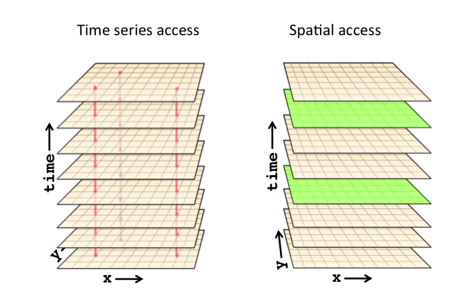
Timeseries

Use the preceding example but extract all data for one single geographical location (pick-up any location).

Solution

from netCDF4 import Dataset    
d = Dataset('large.nc', 'r')
# Do not load dataset yet
data=d.variables['VO']
# pick-up a time and read VO
slice_t=data[:,0,30,30]

The elasped time spent to extract your slice strongly depends on how your data has been stored (how the dimensions are organized):

%matplotlib inline
from netCDF4 import Dataset    
d = Dataset('large.nc', 'r')
# print some metadata
print(d)
d.close()

<class 'netCDF4._netCDF4.Dataset'>
root group (NETCDF3_CLASSIC data model, file format NETCDF3):
    CDI: Climate Data Interface version 1.7.0 (http://mpimet.mpg.de/cdi)
    Conventions: CF-1.4
    history: Thu Feb 04 14:28:54 2016: cdo -t ecmwf -f nc copy EI_VO.grb EI_VO.nc
    institution: European Centre for Medium-Range Weather Forecasts
    CDO: Climate Data Operators version 1.7.0 (http://mpimet.mpg.de/cdo)
    dimensions(sizes): lon(512), lat(256), lev(1), time(200368)
    variables(dimensions): float64 lon(lon), float64 lat(lat), float64 lev(lev), float64 time(time), float32 VO(time,lev,lat,lon)
    groups:

In our case, the time dimension varies most slowly and lon is the fastest.

**Source: http://www.unidata.ucar.edu/blogs/developer/entry/chunking_data_why_it_matters **

The reason is that when storing our dataset, we used the default netCDF storage layout i.e. a conventional contiguous (index-order) storage layout.

So depending on how you want to access (for post-processing or visualization) your data, this may be the best or the worst approach.

A good compromise is the use of chunking, storing multidimensional data in multi-dimensional rectangular chunks to speed up slow accesses at the cost of slowing down fast accesses. Programs that access chunked data can be oblivious to whether or how chunking is used. Chunking is supported in the HDF5 layer of netCDF-4 files, and is one of the features, along with per-chunk compression, that led to a proposal to use HDF5 as a storage layer for netCDF-4 in 2002.

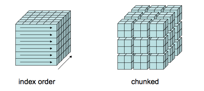
**Source: http://www.unidata.ucar.edu/blogs/developer/entry/chunking_data_why_it_matters **

If you want to learn more on this subject, read this blog here.

Data Tip:

Choose the storage layout that fit your access (read) pattern when post-processing or visualizing data and not when you write. Rewriting data in a different layout can pay off…

netCDF/HDF Data compression

In addition to data chunking, you can compress netCDF/HDF variables on the fly. HDF5 can usually reach easily very good compression level when using szip library (to get this functionality, netCDF-4 and HDF5 need to be compiled with sziplibrary).

Let’s take our previous large.nc file and rewrite it with compression:

%matplotlib inline
import netCDF4 as nc

src_file = 'large.nc'
trg_file = 'large_compressed.nc'
src = nc.Dataset(src_file)
trg = nc.Dataset(trg_file, mode='w')

# Create the dimensions of the file
for name, dim in src.dimensions.items():
    trg.createDimension(name, len(dim) if not dim.isunlimited() else None)

# Copy the global attributes
trg.setncatts({a:src.getncattr(a) for a in src.ncattrs()})

# Create the variables in the file
for name, var in src.variables.items():
    trg.createVariable(name, var.dtype, var.dimensions, zlib=True)

    # Copy the variable attributes
    trg.variables[name].setncatts({a:var.getncattr(a) for a in var.ncattrs()})

    # Copy the variables values (as 'f4' eventually)
    trg.variables[name][:] = src.variables[name][:]

# Save the file
trg.close()
src.close()

Data compression:

Use netCDF-4 / HDF-5 Data compression when writing your dataset to save disk space. NetCDF4 and HDF5 provide easy methods to compress data. When you create variables, you can turn on data compression by setting the keyword argument zlib=True but you can also choose the compression ratio and the precision of your data:

• The complevel keyword argument toggles the compression ratio and speed. Options range from 1 to 9 (1 being the fastest with least compression and 9 being the slowest with most compression. Default is 4).
• The precision of your data can be specified using the least_significant_digit keyword argument. Floats are generally stored with much higher precision than the data it represents, especially if you deal with observed values. Trailing digits take up a lot of space and may not be relevant. By specifying the least significant digit, you can further enhance the data compression. This just gives netCDF more freedom when it packs the data into your harddrive. For instance, knowing that temperature is only accurate to about 0.005 degrees K, it makes sense to just preserve the first 4 digits:

trg.createVariable(name, var.dtype, var.dimensions, zlib=True, least_significant_digit=4)

Recreating the dataset using the above line can significantly reduce the size of your netCDF, especially on large datasets. You can find more information here. And here for HDF5 files; you may also be interested by the two following blogs:

• HDF5 data compression demystified Part-1
• HDF5 Data Compression Demystified Part-2: Performance Tuning

Parallel computing for spatio-temporal data analysis: dask

Dask : a flexible parallel computing library for analytic computing

We usually have large dataset to handle; a lot larger than any examples shown so far in this lesson. Using python as we did so far is not possible any longer:

• our files are too large to fit in memory
• our data processing is too long to be run on a single processor

We have seen that data chunking is very powerful but writing program where we both chunk data and processing can be cumbersome. And to speed-up our processing we need to use more than one processor, so we need a framework which is simple and efficient enough at scale.

Dask is a python library that helps to parallelize computations on big chunks of data. This allows analyzing data that do not fit in to your computer’s memory as well as to utilize multiprocessing capabilities of your machine.

See the very good introduction Dask: Parallel Computing in Python made by Matthew Rocklin at Strata Data Conference 2017.

Let’s see how it works with an example:

%matplotlib inline
import h5py

f = h5py.File('OMI-Aura_L3-OMTO3e_2017m0105_v003-2017m0203t091906.he5', 'r')
dset = f['/HDFEOS/GRIDS/OMI Column Amount O3/Data Fields/ColumnAmountO3']
print(dset.shape)
print(type(dset))

(720, 1440)
<class 'h5py._hl.dataset.Dataset'>

So far, we have just open an HDF5 file with h5py (this package is a very low level API for reading HDF5 files; it is usually very efficient) and read ColumnAmountO3 (Ozone vertical column density). It’s a 2D field, so when we create a dask array, we can split it:

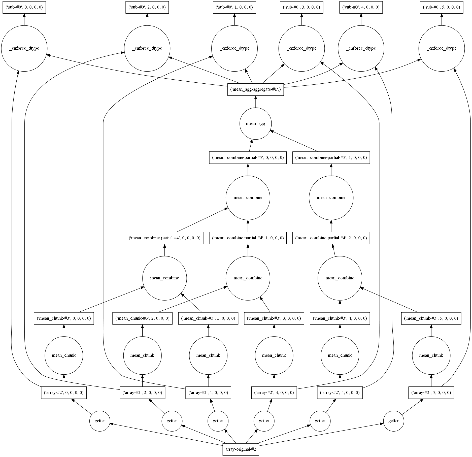
import dask.array as da
d_chunks = da.from_array(dset, chunks=(720, 144))
mx=d_chunks.max()

We haven’t computed anything yet as all operations with dask are deferred. But we can already see the set of operations necessary to compute the maximum value:

mx.visualize()

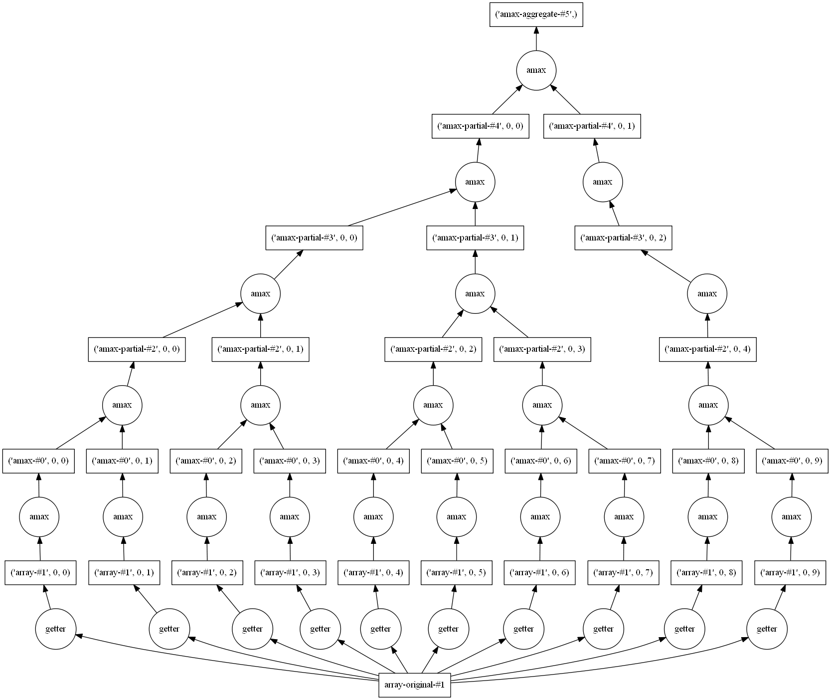
You have to look at the picture from the bottom to the top. At the bottom, you see all your chunks (here 10) and at the top the final result (the maximum value of the entire field).

mx.compute()

512.79999

Here the set of operations is serialized as we do not run it on a multi-processor computer but with significant changes, you could run similar code with large files and on a large number of processors.

And even on your laptop, dask can be very useful because it allows out-of-core operations. This mean that if your file does not fit into the memory of your computer, you still can run large operation on it; but of couse it will be very slow…

Let’s take another example:

%matplotlib inline
import os
import dask.array as da
from netCDF4 import Dataset
from IPython.display import Image

f = Dataset('large.nc')
VO = da.from_array(f.variables['VO'], chunks=(63,1,256,512))
print(VO.shape)
VOmean = VO.mean()   
print(VOmean)
VOmean.visualize()

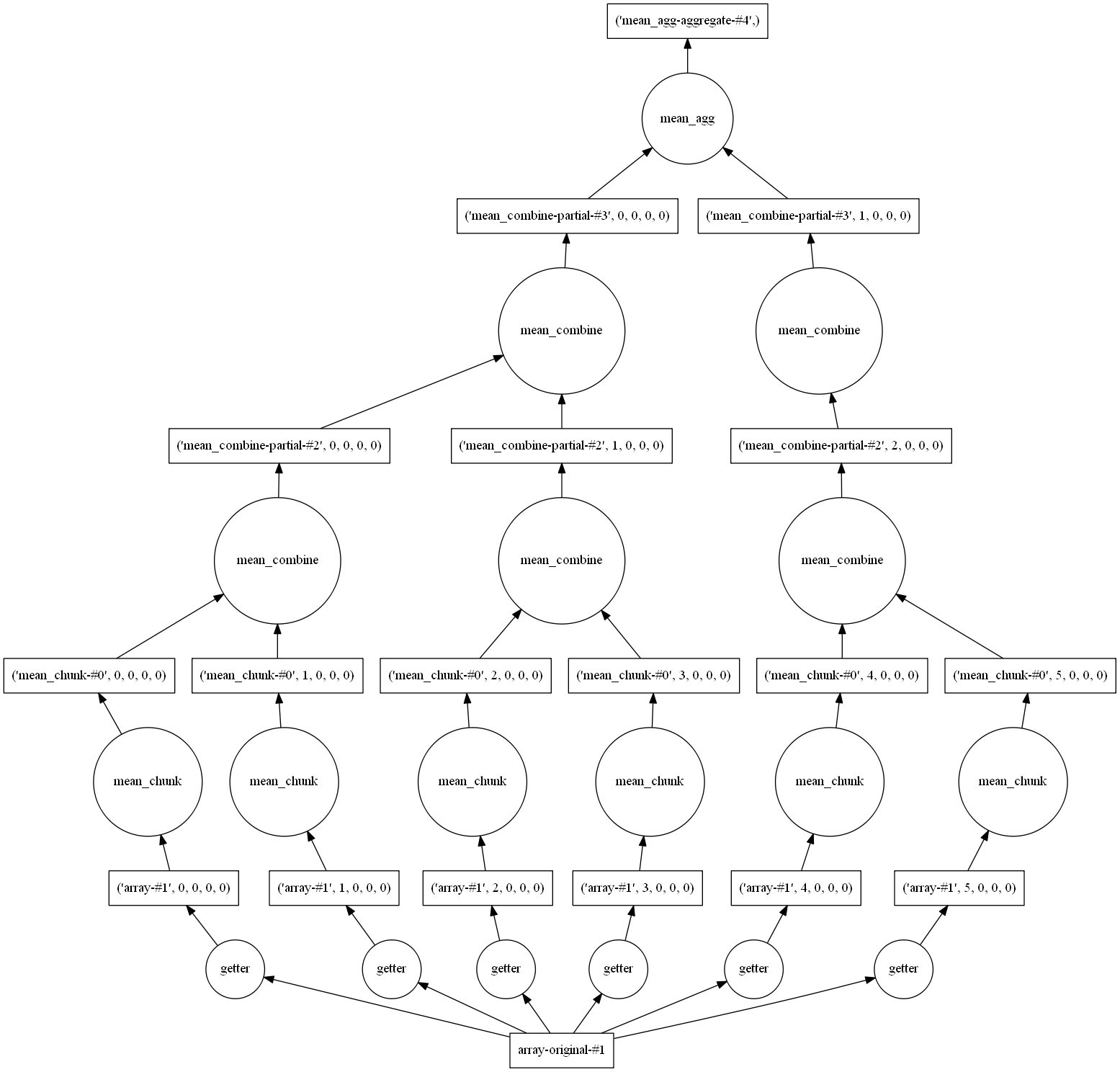
VOmean.compute()

-0.003835564

Use dask to compute standard deviation

Use the same netCDF file and retrieve the average to the original field using dask. Visualize the graph of tasks before computing it.

Solution

(VO - VO.mean()).visualize()
(VO - VO.mean()).compute()

Key Points

• Strategies to manipulate large files in python

• Dask: a flexible parallel computing library for analytic computing