Data Formats in Environmental Sciences

Overview

Teaching: 0 min
Exercises: 0 min

Questions

What are the most common data formats in Environmental Sciences?

raster vs vector formats?

What are the most common python packages to read/write netCDF, HDF, GeoTIFF data files?

Objectives

Learn to recognize the some of the most common data formats in the Environmental sciences.

Learn to open, read and write geoTIFF, netCDF and HDF files

In this lesson we will first review some of the most common spatial data formats used in environmental Sciences and how we categorize them as raster or vector format.
Then we will learn how to recognize raster formats such as GeoTIFF, netCDF and HDF data files.
Finally, we will see what are vector formats and in particular shapefiles.

This lesson is based on the Data Carpentry lesson Geospatial Data Formats.

Types of Spatial Data

Spatial data are represented in many different ways and are stored in different file formats. In this tutorial, we will focus on the two types of spatial data: raster and vector data.

raster data formats

Raster or “gridded” data are saved on a uniform grid and rendered on a map as pixels. Each pixel contains a value that represents an area on the Earth’s surface.

raster concept

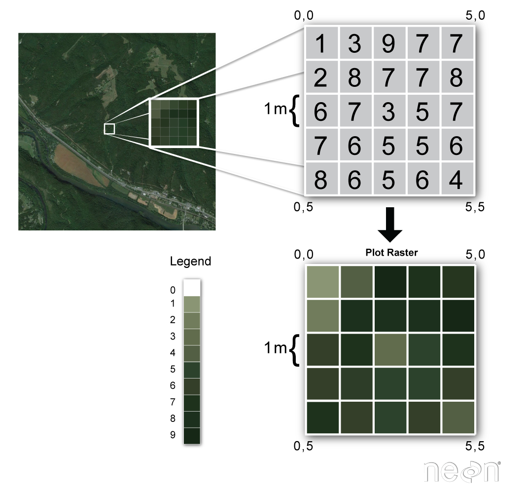
Source: National Ecological Observatory Network (NEON)

There are many different raster data file formats. In this lesson, we will focus on the

netCDF data format
HDF data format
GeoTIFF data format

netCDF

NetCDF (network Common Data Form) is a:

Self-Describing
Portable
Scalable
Appendable
Sharable
Archivable

data format standard for exchanging scientific data.

Self-describing?	Portable?	Scalable?	Appendable?	Sharable?	Archivable?
Information describing the data contents of the file are embedded within the data file itself. This means that there is a header which describes the layout of the rest of the file, in particular the data arrays, as well as arbitrary file metadata in the form of name/value attributes.	A NetCDF file is machine-independent i.e. it can be accessed by computers with different ways of storing integers, characters, and floating-point numbers.For instance, issues such as endianness being addressed in the software libraries.	A small subset of a large dataset may be accessed efficiently.	Data may be appended to a properly structured NetCDF file without copying the dataset or redefining its structure.	One writer and multiple readers may simultaneously access the same NetCDF file.	Access to all earlier forms of NetCDF data will be supported by current and future versions of the software.

The netCDF project homepage is hosted by the Unidata program at the University Corporation for Atmospheric Research (UCAR).

As all self-describing data formats, netCDF includes a standard API (Application program interface) and portable data access libraries in a variety of languages, including python. There are netCDF tools that can open and work with arbitrary netCDF files, using the embedded descriptions to interpret the data.

What does it really mean when we say that a netCDF file is self-describing? Let’s find out with an example “MITgcm_state.nc”. If you do not have downloaded the metos_python data for this lesson, please see the setup instructions).

In this example, we will be looking at the metadataof a netCDF file. For this we open the netCDF file with the netCDF4 python package you were asked to install.

from netCDF4 import Dataset
nc_f = 'tpw_v07r01_200910.nc4.nc'  # Your filename
nc_fid = Dataset(nc_f, 'r')  # Dataset is the class behavior to open the file
                             # and create an instance of the ncCDF4 class
print(nc_fid)
nc_fid.close()

<class 'netCDF4._netCDF4.Dataset'>
root group (NETCDF4 data model, file format HDF5):
    Conventions: CF-1.6
    title: Monthly mean total precipitable water (total column water vapor) and anomalies on a 1.0 degree grid made from RSS Version-7 microwave radiometer data
    institution: Remote Sensing Systems
    source: Satellite Microwave Radiometer brightness temperatures converted to precipitable water using RSS Version-7 algorithm
    references: More information is available at http://www.remss.com/measurements/atmospheric-water-vapor/tpw-1-deg-product ; See also Wentz, FJ, L Ricciardulli, KA Hilburn and others, 2007, How much more rain will global warming bring?, Science, 317, 233-235, and Wentz, FJ, MC Schabel, 2000, Precise climate monitoring using complementary satellite data sets, Nature, 403, 414-416.
    history: 2012, Carl A Mears, Remote Sensing Systems, data set created from V-7 DISCOVER satellite microwave vapor data
    Metadata_Conventions: CF-1.6, Unidata Dataset Discovery v1.0, NOAA CDR v1.0, GDS v2.0
    standard_name_vocabulary: CF Standard Name Table (v19, 22 March 2012)
    id: tpw_v07r01_200910.nc4.nc
    naming_authority: www.remss.com
    date_created: 2016-04-13T19:05:12Z
    license: No constraints on data access or use
    summary: Gridded monthly means and anomalies of total precipitable water (total column water vapor) from SSM/I, SSMIS, AMSRE, WindSat, and AMSR2 microwave radiometers processed with Version-7 algorithm
    keywords: Atmosphere > Atmospheric Water Vapor > Precipitable Water
    keywords_vocabulary: NASA Global Change Master Directory (GCMD) Earth Science keywords, Version 6.0
    cdm_data_type: Grid
    project: NASA MEaSUREs funded DISCOVER project
    processing_level: NASA EOSDIS Data Level 4
    creator_name: Frank J. Wentz, PI DISCOVER Project, Remote Sensing Systems
    creator_url: http://www.remss.com/
    creator_email: support@remss.com
    geospatial_lat_min: -90.0
    geospatial_lat_max: 90.0
    geospatial_lon_min: 0.0
    geospatial_lon_max: 360.0
    geospatial_lat_units: degrees_north
    geospatial_lon_units: degrees_east
    geospatial_lat_resolution: 1.0
    geospatial_lon_resolution: 1.0
    time_coverage_start: 2009-10-01T00:00:00Z
    time_coverage_end: 2009-10-31T23:59:59Z
    time_coverage_duration: P1M
    time_coverage_resolution: P1M
    contributor_name: Frank J. Wentz, Carl A. Mears, Deborah K Smith, Marty Brewer
    contributor_role: principalInvestigator, author/processor, pointOfContact, processor
    acknowledgement: Microwave radiometer data are processed by Remote Sensing Systems with funding from the NASA Earth Science MEaSUREs Program and the NASA Earth Science Physical Oceanography Program.
    product_version: V7.0
    platform: DMSP-F08,DMSP-F10,DMSP-F11,DMSP-F13,DMSP-F14,DMSP-F15,DMSP-F16,DMSP-F17,AQUA,Coriolis,GCOM-W1
    sensor: DMSP F08-F15 > SSM/I, DMSP F16-F17 > SSMIS, AQUA > AMSRE, Coriolis > WindSat, GCOM-W > AMSR2
    spatial_resolution: 1.0 degree
    comment: In precipitable_water and precipitable_water_anomaly, Missing data and land denoted by -999.0.  Ice is denoted by -500.0.  In other variables, missing data, land and ice are all denoted by -999.0.
    identifier_product_DOI_authority: http://dx.doi.org/
    identifier_product_DOI: http://dx.doi.org/10.5067/MEASURES/MULTIPLE/WATER_VAPOR/DATA301
    provenance: Subset from tpw_v07r01_198801_201603.nc4.nc on host gale in the ops environment on 2016-04-13T19:05:12Z
    dimensions(sizes): longitude(360), latitude(180), time(1), climatology_time(12), satnum(11), bnds(2)
    variables(dimensions): float32 longitude(longitude), float32 latitude(latitude), int32 time(time), <class 'str'> platform_names(satnum), float32 longitude_bounds(longitude,bnds), float32 latitude_bounds(latitude,bnds), float32 time_bounds(time,bnds), float32 precipitable_water(time,latitude,longitude), float32 precipitable_water_anomaly(time,latitude,longitude), int8 satellites_used(time,satnum), float32 global_mean_precipitable_water_anomaly(time), float32 tropical_mean_precipitable_water_anomaly(time)
    groups: 

Check a netCDF file?

Most of the time, netCDF filename extensions are either .nc or .nc4. However, it is not a mandatory requirement so it is useful to learn to check if a file is a netCDF file:

$ file tpw_v07r01_200910.nc4.nc

tpw_v07r01_200910.nc4.nc: NetCDF Data Format data

file is a bash shell command and is not a netCDF utility. You can use it for any kind of files and it attempts torecognize its data format.

netCDF and python?

The most common low-level python packages to handle netcdf is called netcdf4 python package. The functionalities covered by this python package are close to those covered by Unidata netCDF library.

Start a new jupyter notebook and enter:

import netCDF4

Creating netCDF files

All of the following code examples assume that the netcdf4-python library has been imported:

import netCDF4

Then 4 following steps:

Dataset and Files
Dimensions
Variables
Writing and Retrieving data

Create an empty netCDF4 dataset and store it on disk

foo = netCDF4.Dataset('foo.nc', 'w')
foo.close()

Then you should find a new file called “foo.nc” in your working directory:

ls

foo.nc

The Dataset constructor defaults to creating NETCDF4 format objects. Other formats may be specified with the format keyword argument (see the netCDF4-python docs).

The first argument that Dataset takes is the path and name of the netCDF4 file that will be created, updated, or read. The second argument is the mode with which to access the file. Use:

w (write mode) to create a new file, use clobber=True to over-write and existing one
r (read mode) to open an existing file read-only
r+ (append mode) to open an existing file and change its contents

Dimensions

Create dimensions on a dataset with the createDimension() method. We first create a new netCDF file but this time we don’t close it immediately and create 3 dimensions:

import netCDF4
f = netCDF4.Dataset('orography.nc', 'w')
f.createDimension('time', None)
f.createDimension('z', 3)
f.createDimension('y', 4)
f.createDimension('x', 5)

The first dimension is called time with unlimited size (i.e. variable values may be appended along the this dimension). Unlimited size dimensions must be declared before (“to the left of”) other dimensions. We usually use only a single unlimited size dimension that is used for time.

The other 3 dimensions are spatial dimensions with sizes of 3, 4, and 5, respectively.

The recommended maximum number of dimensions is 4. The recommended order of dimensions is time, z, y, x. Not all datasets are required to have all 4 dimensions.

Variables

Create variables on a dataset with the createVariable() method, for example:

lats = f.createVariable('lat', float, ('y', ), zlib=True)
lons = f.createVariable('lon', float, ('x', ), zlib=True)
orography = f.createVariable('orog', float, ('y', 'x'), zlib=True, least_significant_digit=1, fill_value=0)
f.close()

The first argument to createVariable() is the variable name.

The second argument is the variable type. There are many way of specifying type, but Python built-in types work well in the absence of specific requirements.

The third argument is a tuple of previously defined dimension names. As noted above,

The recommended maximum number of dimensions is 4 The recommended order of dimensions is t, z, y, x Not all variables are required to have all 4 dimensions All variables should be created with the zlib=True argument to enable data compression within the netCDF4 file.

When appropriate, the least_significant_digit argument should be used to improve compression and storage efficiency by quantizing the variable data to the specified precision. In the example above the orography data will be quantized such that a precision of 0.1 is retained.

When appropriate, the fill_value argument can be used to specify the value that the variable gets filled with before any data is written to it. Doing so overrides the default netCDF _FillValue (which depends on the type of the variable). If fill_value is set to False, then the variable is not pre-filled.

In the example above the orography data will be initialized to zero, the appropriate value for grid points that are over ocean.

Writing and Retrieving Data

Writing Data

Variable data in netCDF4 datasets are stored in NumPy array or masked array objects.

An appropriately sized and shaped NumPy array can be loaded into a dataset variable by assigning it to a slice that span the variable:

import netCDF4
import numpy as np

f = netCDF4.Dataset('orography.nc', 'w')
f.createDimension('time', None)
f.createDimension('z', 3)
f.createDimension('y', 4)
f.createDimension('x', 5)
lats = f.createVariable('lat', float, ('y', ), zlib=True)
lons = f.createVariable('lon', float, ('x', ), zlib=True)
orography = f.createVariable('orog', float, ('y', 'x'), zlib=True, least_significant_digit=1, fill_value=0)
# create latitude and longitude 1D arrays
lat_out  = [60, 65, 70, 75]
lon_out  = [ 30,  60,  90, 120, 150]
# Create field values for orography
data_out = np.arange(4*5) # 1d array but with dimension x*y
data_out.shape = (4,5)    # reshape to 2d array
orography[:] = data_out
lats[:] = lat_out
lons[:] = lon_out
# close file to write on disk
f.close()

We defined a one-dimensional array data_out and reshape it to a 2 dimensional array and then store it in the orography netCDF variable.

Let’s have look to the netCDF file we generated and in particular its metadata:

import netCDF4
f = netCDF4.Dataset('orography.nc', 'r')
print(f)
f.close()

<class 'netCDF4._netCDF4.Dataset'>
root group (NETCDF4 data model, file format HDF5):
    dimensions(sizes): time(0), z(3), y(4), x(5)
    variables(dimensions): float64 lat(y), float64 lon(x), float64 orog(y,x)
    groups: 

Understand netCDF file

Check the orography.nc file:

What is the first value of the orog variable?

What is the missing value for lat and lon variables?

Solution

The first value of orog is 0 but it appears as “_” which corresponds to a missing value (also called filled value). When we defined orog variable, we set its filled/missing value to 0. Therefore, every occurence of 0 will be flagged as a missing value.

We haven’t specified any filled values for lat and lon so default missing values are set by default, depending on the type of variable; here lat and lon were defined as float so the default missing value is 9.969209968386869e+36. You can check the netCDF4 default filled values: netCDF4.default_fillvals

Retrieve Data

Let’s first read the file we previously generated:

import netCDF4
import numpy as np

f = netCDF4.Dataset('orography.nc', 'r')
lats = f.variables['lat']
lons = f.variables['lon']
orography = f.variables['orog']
print(lats[:])
print(lons[:])
print(orography[:])
f.close()

lats vs. lats[:]?

What is the type of lats?

What is the difference between lats and lats[:]?

Solution

lats is a netCDF variable: ` type(lats)returns:<class ‘netCDF4._netCDF4.Variable’>`

lats is a netCDF variable; a lot more than a simple numpy array while lats[:] allows you to access the latitudes values stored in the lats netCDF variable. lats[:] is a numpy array.

Values can be retrieved using most of the usual NumPy indexing and slicing techniques.

However, there are differences between the NumPy and netCDF variable slicing rules; see the netCDF4-python docs for details.

Now if we only want to access a subset of the variable orog:

import netCDF4
import numpy as np

f = netCDF4.Dataset('orography.nc', 'r')
lats = f.variables['lat']
lons = f.variables['lon']
orography = f.variables['orog']
print(lats[:])
print(lons[:])
print(orography[:][3,2])
f.close()

Types of netCDF files?

There are four NetCDF format variants according to the Unidata NetCDF FAQ page:

the classic format,

the 64-bit offset format,

the NetCDF-4 format, and

the NetCDF-4 classic model format. While this seems to add even more complexity to using NetCDF files, the reality is that unless you are generating NetCDF files, most applications read NetCDF files regardless of type with no issues. This aspect has been abstracted for the general user!

The classic format has its roots in the original version of the NetCDF standard. It is the default for new files.

The 64-bit offset simply allows for larger dataset to be created. Prior to the offset, files would be limited to 2 GB. A 64-bit machine is not required to read a 64-bit file. This point should not be a concern for many users.

The NetCDF-4 format adds many new features related to compression and multiple unlimited dimensions. NetCDF-4 is essentially a special case of the HDF5 file format. netCDF4 is and extension to the classic model often called netCDF3. netCDF4 adds more powerful forms of data representation and data types at the expense of some additional complexity; it is based on HDF and therefore requires the installation of the HDF libraries prior to the installation of netCDF. It you installed netCDF without having HDF libraries on your machine, then you probably only have netCDF3.

The NetCDF-4 classic model format attempts to bridge gaps between the original NetCDF file and NetCDF-4.

Luckily for us, the NetCDF4 Python module handles many of these differences.

CF conventions?

netCDF format is self-describing but very flexible and you still have to decide how to encode your data into the format:

Layout of data within the file
Unambiguous names for fields; Use standard names if possible
Units
Fill/missing values

Therefore to simplify developments of tools and speed-up netCDF data processing, metadata standards for netCDF files have been created. The most common in our discipline is the Climate and Forecast metadata standard, also called CF conventions.

The CF conventions have been adopted by the Program for Climate Model Diagnosis and Intercomparison (PCMDI), the Earth System Modeling Framework (ESMF), NCAR, and various EU and international projects.

If you plan to create netCDF files, following CF conventions is recommended. However, if you are curious or encounter data using a different convention, Unidata maintains a list you can use to find out more information.

Let’s have a look at a netCDF file called sresa1b_ncar_ccsm3-example.nc that follows CF conventions. If you haven’t downloaded this file, see the setup instructions:

import netCDF4
f = netCDF4.Dataset("sresa1b_ncar_ccsm3-example.nc", "r")
print(f)
f.close()

<class 'netCDF4._netCDF4.Dataset'>
root group (NETCDF3_CLASSIC data model, file format NETCDF3):
    CVS_Id: $Id$
    creation_date: 
    prg_ID: Source file unknown Version unknown Date unknown
    cmd_ln: bds -x 256 -y 128 -m 23 -o /data/zender/data/dst_T85.nc
    history: Tue Oct 25 15:08:51 2005: ncks -O -x -v va -m sresa1b_ncar_ccsm3_0_run1_200001.nc sresa1b_ncar_ccsm3_0_run1_200001.nc
Tue Oct 25 15:07:21 2005: ncks -d time,0 sresa1b_ncar_ccsm3_0_run1_200001_201912.nc sresa1b_ncar_ccsm3_0_run1_200001.nc
Tue Oct 25 13:29:43 2005: ncks -d time,0,239 sresa1b_ncar_ccsm3_0_run1_200001_209912.nc /var/www/html/tmp/sresa1b_ncar_ccsm3_0_run1_200001_201912.nc
Thu Oct 20 10:47:50 2005: ncks -A -v va /data/brownmc/sresa1b/atm/mo/va/ncar_ccsm3_0/run1/sresa1b_ncar_ccsm3_0_run1_va_200001_209912.nc /data/brownmc/sresa1b/atm/mo/tas/ncar_ccsm3_0/run1/sresa1b_ncar_ccsm3_0_run1_200001_209912.nc
Wed Oct 19 14:55:04 2005: ncks -F -d time,01,1200 /data/brownmc/sresa1b/atm/mo/va/ncar_ccsm3_0/run1/sresa1b_ncar_ccsm3_0_run1_va_200001_209912.nc /data/brownmc/sresa1b/atm/mo/va/ncar_ccsm3_0/run1/sresa1b_ncar_ccsm3_0_run1_va_200001_209912.nc
Wed Oct 19 14:53:28 2005: ncrcat /data/brownmc/sresa1b/atm/mo/va/ncar_ccsm3_0/run1/foo_05_1200.nc /data/brownmc/sresa1b/atm/mo/va/ncar_ccsm3_0/run1/foo_1192_1196.nc /data/brownmc/sresa1b/atm/mo/va/ncar_ccsm3_0/run1/sresa1b_ncar_ccsm3_0_run1_va_200001_209912.nc
Wed Oct 19 14:50:38 2005: ncks -F -d time,05,1200 /data/brownmc/sresa1b/atm/mo/va/ncar_ccsm3_0/run1/va_A1.SRESA1B_1.CCSM.atmm.2000-01_cat_2099-12.nc /data/brownmc/sresa1b/atm/mo/va/ncar_ccsm3_0/run1/foo_05_1200.nc
Wed Oct 19 14:49:45 2005: ncrcat /data/brownmc/sresa1b/atm/mo/va/ncar_ccsm3_0/run1/va_A1.SRESA1B_1.CCSM.atmm.2000-01_cat_2079-12.nc /data/brownmc/sresa1b/atm/mo/va/ncar_ccsm3_0/run1/va_A1.SRESA1B_1.CCSM.atmm.2080-01_cat_2099-12.nc /data/brownmc/sresa1b/atm/mo/va/ncar_ccsm3_0/run1/va_A1.SRESA1B_1.CCSM.atmm.2000-01_cat_2099-12.nc
Created from CCSM3 case b30.040a
 by wgstrand@ucar.edu
 on Wed Nov 17 14:12:57 EST 2004
 
 For all data, added IPCC requested metadata
    table_id: Table A1
    title: model output prepared for IPCC AR4
    institution: NCAR (National Center for Atmospheric 
Research, Boulder, CO, USA)
    source: CCSM3.0, version beta19 (2004): 
atmosphere: CAM3.0, T85L26;
ocean     : POP1.4.3 (modified), gx1v3
sea ice   : CSIM5.0, T85;
land      : CLM3.0, gx1v3
    contact: ccsm@ucar.edu
    project_id: IPCC Fourth Assessment
    Conventions: CF-1.0
    references: Collins, W.D., et al., 2005:
 The Community Climate System Model, Version 3
 Journal of Climate
 
 Main website: http://www.ccsm.ucar.edu
    acknowledgment:  Any use of CCSM data should acknowledge the contribution
 of the CCSM project and CCSM sponsor agencies with the 
 following citation:
 'This research uses data provided by the Community Climate
 System Model project (www.ccsm.ucar.edu), supported by the
 Directorate for Geosciences of the National Science Foundation
 and the Office of Biological and Environmental Research of
 the U.S. Department of Energy.'
In addition, the words 'Community Climate System Model' and
 'CCSM' should be included as metadata for webpages referencing
 work using CCSM data or as keywords provided to journal or book
publishers of your manuscripts.
Users of CCSM data accept the responsibility of emailing
 citations of publications of research using CCSM data to
 ccsm@ucar.edu.
Any redistribution of CCSM data must include this data
 acknowledgement statement.
    realization: 1
    experiment_id: 720 ppm stabilization experiment (SRESA1B)
    comment: This simulation was initiated from year 2000 of 
 CCSM3 model run b30.030a and executed on 
 hardware cheetah.ccs.ornl.gov. The input external forcings are
ozone forcing    : A1B.ozone.128x64_L18_1991-2100_c040528.nc
aerosol optics   : AerosolOptics_c040105.nc
aerosol MMR      : AerosolMass_V_128x256_clim_c031022.nc
carbon scaling   : carbonscaling_A1B_1990-2100_c040609.nc
solar forcing    : Fixed at 1366.5 W m-2
GHGs             : ghg_ipcc_A1B_1870-2100_c040521.nc
GHG loss rates   : noaamisc.r8.nc
volcanic forcing : none
DMS emissions    : DMS_emissions_128x256_clim_c040122.nc
oxidants         : oxid_128x256_L26_clim_c040112.nc
SOx emissions    : SOx_emissions_A1B_128x256_L2_1990-2100_c040608.nc
 Physical constants used for derived data:
 Lv (latent heat of evaporation): 2.501e6 J kg-1
 Lf (latent heat of fusion     ): 3.337e5 J kg-1
 r[h2o] (density of water      ): 1000 kg m-3
 g2kg   (grams to kilograms    ): 1000 g kg-1
 
 Integrations were performed by NCAR and CRIEPI with support
 and facilities provided by NSF, DOE, MEXT and ESC/JAMSTEC.
    model_name_english: NCAR CCSM
    dimensions(sizes): lat(128), lon(256), bnds(2), plev(17), time(1)
    variables(dimensions): float32 area(lat,lon), float32 lat(lat), float64 lat_bnds(lat,bnds), float32 lon(lon), float64 lon_bnds(lon,bnds), int32 msk_rgn(lat,lon), float64 plev(plev), float32 pr(time,lat,lon), float32 tas(time,lat,lon), float64 time(time), float64 time_bnds(time,bnds), float32 ua(time,plev,lat,lon)
    groups:

HDF

Hierarchical Data Format (HDF) is a data file format designed by the National Center for Supercomputing Applications (NCSA).

It is now developed and maintained by the HDF group.

Hierarchical Data Format, commonly abbreviated HDF, HDF4, or HDF5, is a library and multi-object file format for the transfer of graphical and numerical data between computers.

HDF supports several different data models, including multidimensional arrays, raster images, and tables. Each defines a specific aggregate data type and provides an API for reading, writing, and organising the data and metadata. New data models can be added by the HDF developers or users.

HDF is self-describing, allowing an application to interpret the structure and contents of a file without any outside information. One HDF file can hold a mixture of related objects, which can be accessed as a group or as individual objects.

Check an HDF file?

The file (the MISR Level 3 Land products May 2007) we will be using has been downloaded at https://l0dup05.larc.nasa.gov/L3Web/download. You first need to register (free registration) to download data from this link and for this tutorial, we have included a copy in the tutorial dataset.

$ file MISR_AM1_CGLS_MAY_2007_F04_0031.hdf

MISR_AM1_CGLS_MAY_2007_F04_0031.hdf: Hierarchical Data Format (version 4) data

Note that in addition it gives some information on the version (4). The HDF version may be important as we will explain later in this lesson.

HDF data files and python?

If you are using python anaconda, HDF files can be accessed in python using the netCDF4 python package, exactly as netCDF files. The reason is that netCDF files (netCDF4) is based on HDF5. pyhdf is also a very well know python package used to access HDF files. However, in this lesson we will only show how to handle HDF files with netCDF4 python package.

Let’s first look at MISR_AM1_CGLS_MAY_2007_F04_0031.hdf and gets metadata:

from netCDF4 import Dataset

f=Dataset('MISR_AM1_CGLS_MAY_2007_F04_0031.hdf','r')
print("Metadata for the dataset:")
print(f)
print("List of available variables (or key): ")
f.variable.keys()
print("Metadata for 'NDVI average' variable: ")
f.variables["NDVI average"]
f.close()

Quick visualization with Python

We will see later how to customize our plots and make geographical maps but for now we just want to get a quick overview of our data with python using imshow from the matplotlib package.

%matplotlib inline
from netCDF4 import Dataset
import matplotlib.pyplot as plt

f=Dataset('MISR_AM1_CGLS_MAY_2007_F04_0031.hdf','r')
data=f.variables['NDVI average'][:]
print(type(data))
print(data.shape)
plt.imshow(data)
plt.show()
f.close()

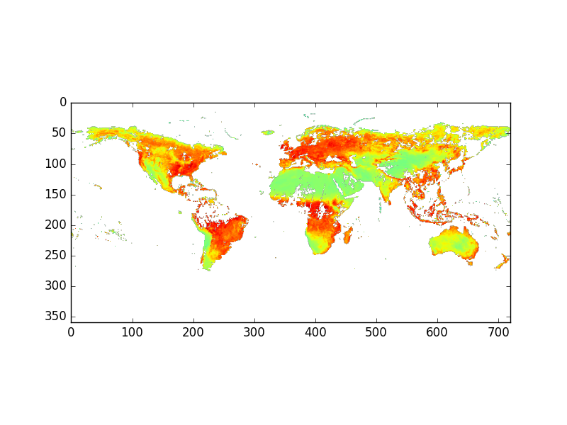
NDVI average May 2007 (MISR Level 3 Land products)

We are using matplotlib, the most common 2D plotting python package. Many other plotting python packages make use of matplotlib and offer to users higher-level user interface. This is why it is always useful to know about matplotlib.

Types of HDF files?

There are two versions of HDF technologies that are completely different: HDF4 and HDF5. HDF4 is the first HDF format. The HDF5 Format is completely different from HDF4 and different libraries are required to read/write these two different formats. Hopefully, the NetCDF4 Python module handles many of these differences. Nowadays, when we refer to HDF files, we often mean HDF5 data files.

EOS Conventions?

HDF-EOS is an extension of HDF4. On December 18, 1999, NASA and its international partners launched Terra, the first of the Earth Observing System (EOS) satellites planned for NASA’s Earth Science Enterprise (ESE) program. Although HDF meets many NASA specifications for accessing data, EOS applications required additional conventions and data types, which led to the development of HDF-EOS based on HDF4.

Tools for handling HDF-EOS can be found at the HDF-EOS Tools and Information Centre.

In 2007, HDF-EOS5 Data Model File Format became an approved standard recommended for use in NASA Earth Science Data Systems. As for HDF-EOS, it is an extension of HDF but it is now based on HDF5.

HDF4 or HDF5?

The examples used in the following exercises are HDF files downloaded at http://hdfeos.org/zoo/index_openGESDISC_Examples.php.

What is the type of OMI-Aura_L3-OMTO3e_2017m0105_v003-2017m0203t091906.he5 and AIRS.2002.08.30.227.L2.RetStd_H.v6.0.12.0.G14101125810.hdf?
Solution
OMI-Aura_L3-OMTO3e_2017m0105_v003-2017m0203t091906.he5 is an HDF5 file and more precisely HDF-EOS5 while AIRS.2002.08.30.227.L2.RetStd_H.v6.0.12.0.G14101125810.hdf is and HDF4 file. You can check either using the file command or in python:
from netCDF4 import Dataset
f = Dataset('data/OMI-Aura_L3-OMTO3e_2017m0105_v003-2017m0203t091906.he5')
print(f)
f.close()
<class 'netCDF4._netCDF4.Dataset'>
root group (NETCDF4 data model, file format HDF5):
   dimensions(sizes): 
   variables(dimensions): 
   groups: HDFEOS, HDFEOS INFORMATION
file AIRS.2002.08.30.227.L2.RetStd_H.v6.0.12.0.G14101125810.hdf
AIRS.2002.08.30.227.L2.RetStd_H.v6.0.12.0.G14101125810.hdf: Hierarchical Data Format (version 4) data

Quick plot with imshow

The examples used in the following exercises are HDF files downloaded at http://hdfeos.org/zoo/index_openGESDISC_Examples.php.

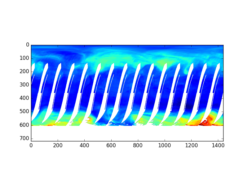
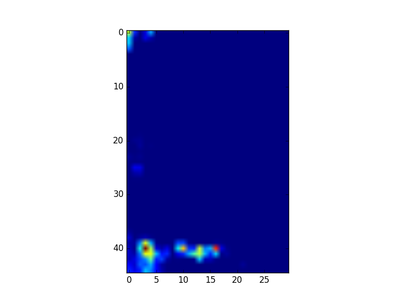
Write a python program using imshow to visualize the 2D variable ColumnAmountO3 from OMI-Aura_L3-OMTO3e_2017m0105_v003-2017m0203t091906.he5?

Do the same for the variable called topog for AIRS.2002.08.30.227.L2.RetStd_H.v6.0.12.0.G14101125810.hdf?
Solution
%matplotlib inline
from netCDF4 import Dataset
import matplotlib.pyplot as plt
f = Dataset('data/OMI-Aura_L3-OMTO3e_2017m0105_v003-2017m0203t091906.he5')
data = f.groups['HDFEOS'].groups['GRIDS'].groups['OMI Column Amount O3'].groups['Data Fields'].variables['ColumnAmountO3']
plt.imshow(data)
plt.show()
f.close()
2.
%matplotlib inline
from netCDF4 import Dataset
f = Dataset('AIRS.2002.08.30.227.L2.RetStd_H.v6.0.12.0.G14101125810.hdf')
data = f.variables['topog']
plt.imshow(data)
plt.show()
f.close()

GeoTIFF

TIFF (Tagged Image File Format) is a raster file format for digital images, created by Aldus Corporation (merged later with Adobe) widely used for raster imagery and aerial photoraphy.

A GeoTIFF file is a georeferenced TIFF, which means it can have geographic information such as map projections embedded within the header file of the TIFF itself.

This means that a GIS application can position the image in the correct location.

Strictly speaking, GeoTIFF is a metadata format, but the TIFF format enables both the data and metadata to exist in the same file.

GeoTIFFs are commonly used for a range of raster data, including:

remote sensing & aerial photography;
satellite data;
cartographic representations, such as georeferenced topomaps.

GeoTIFFs are also often supported by GPS units.

Let’s take an example; a GeoTIFF MODIS image showing Southern Norway and Sweden (date: 16/08/2017) with True Color:

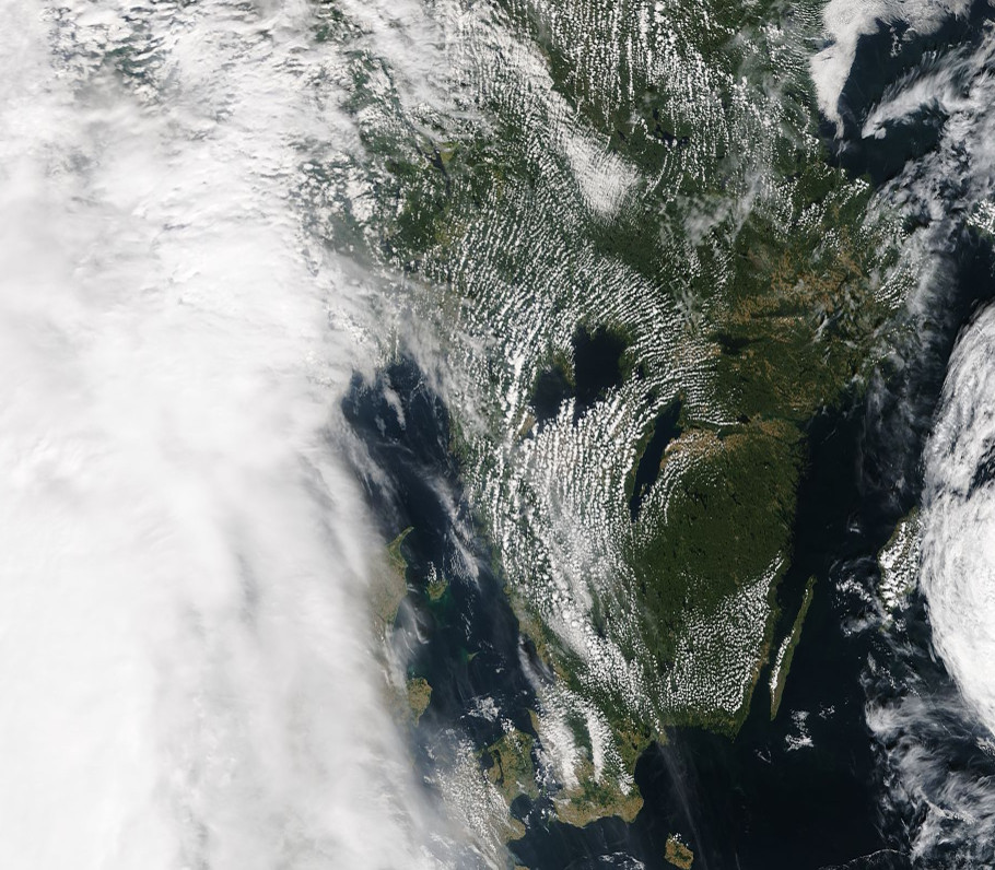
MODIS Aqua 1km over Southern Norway and Sweden

Source: MODIS Aqua 1km over Southern Norway and Sweden

We cannot use netCDF4 python package to read/write GeoTIFF data files but we can use the Geospatial Data Abstraction Library (GDAL) tools and library to inspect this file. This additional package needs to be installed (see setup instructions). This library is very powerful and can read/write most raster data formats, including netCDF and HDF. It means that the example we will be given for reading GeoTIFF files can also be applied to read the netCDF and HDF files we used in this lesson. See the list of data formats GDAL can handle here.

from osgeo import gdal
datafile = gdal.Open('metos_python/data/Southern_Norway_and_Sweden.2017229.terra.1km.tif')
print( "Driver: ",datafile.GetDriver().ShortName, datafile.GetDriver().LongName)
print( "Size is ", datafile.RasterXSize, datafile.RasterYSize)
print( "Bands = ", datafile.RasterCount)
print( "Coordinate System is:", datafile.GetProjectionRef ())
print( "GetGeoTransform() = ", datafile.GetGeoTransform ())
print( "GetMetadata() = ", datafile.GetMetadata ())

Driver:  GTiff GeoTIFF
Size is  910 796
Bands =  3
Coordinate System is: GEOGCS["WGS 84",DATUM["WGS_1984",SPHEROID["WGS 84",6378137,298.257223563,AUTHORITY["EPSG","7030"]],AUTHORITY["EPSG","6326"]],PRIMEM["Greenwich",0],UNIT["degree",0.0174532925199433],AUTHORITY["EPSG","4326"]]
GetGeoTransform() =  (4.0, 0.017582417582417617, 0.0, 62.0, 0.0, -0.008793969849246248)
GetMetadata() =  {'AREA_OR_POINT': 'Area', 'TIFFTAG_SOFTWARE': 'ppm2geotiff v0.0.9'}

On Linux or Mac OSX, you can also use gdalinfo command line to get similar information:

gdalinfo metos_python/data/Southern_Norway_and_Sweden.2017229.terra.1km.tif

Driver: GTiff/GeoTIFF
Files: Southern_Norway_and_Sweden.2017229.terra.1km.tif
Size is 910, 796
Coordinate System is:
GEOGCS["WGS 84",
    DATUM["WGS_1984",
        SPHEROID["WGS 84",6378137,298.257223563,
            AUTHORITY["EPSG","7030"]],
        AUTHORITY["EPSG","6326"]],
    PRIMEM["Greenwich",0],
    UNIT["degree",0.0174532925199433],
    AUTHORITY["EPSG","4326"]]
Origin = (4.000000000000000,62.000000000000000)
Pixel Size = (0.017582417582418,-0.008793969849246)
Metadata:
  AREA_OR_POINT=Area
  TIFFTAG_SOFTWARE=ppm2geotiff v0.0.9
Image Structure Metadata:
  INTERLEAVE=PIXEL
Corner Coordinates:
Upper Left  (   4.0000000,  62.0000000) (  4d 0' 0.00"E, 62d 0' 0.00"N)
Lower Left  (   4.0000000,  55.0000000) (  4d 0' 0.00"E, 55d 0' 0.00"N)
Upper Right (  20.0000000,  62.0000000) ( 20d 0' 0.00"E, 62d 0' 0.00"N)
Lower Right (  20.0000000,  55.0000000) ( 20d 0' 0.00"E, 55d 0' 0.00"N)
Center      (  12.0000000,  58.5000000) ( 12d 0' 0.00"E, 58d30' 0.00"N)
Band 1 Block=910x3 Type=Byte, ColorInterp=Red
Band 2 Block=910x3 Type=Byte, ColorInterp=Green
Band 3 Block=910x3 Type=Byte, ColorInterp=Blue

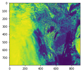
This GeoTIFF file contains 3 bands (Red, Green and Blue), so we can extract each band and visualize one band with imshow:

bnd1 = datafile.GetRasterBand(1).ReadAsArray()
bnd2 = datafile.GetRasterBand(2).ReadAsArray()
bnd3 = datafile.GetRasterBand(3).ReadAsArray()

plt.imshow(bnd1)
plt.show()

raster concept

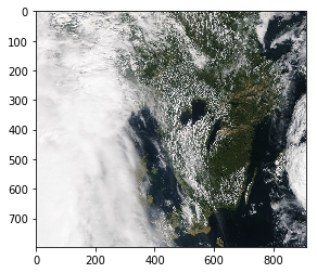
To visualize our 3 bands as an RGB image, we need to stack the 3 indivual arrays into one image:

print(type(bnd1), bnd1.shape)
print(type(bnd2), bnd3.shape)
print(type(bnd3), bnd3.shape)
img = np.dstack((bnd1,bnd2,bnd3))
print(type(img), img.shape)
plt.imshow(img)
plt.show()

raster concept

vector data formats

Vector data are very common and efficient geospatial formats and are often used to store things like road and plot locations, boundaries of states, countries and lakes.

Vector data are composed of discrete geometric locations (x,y values) known as vertices that define the “shape” of the spatial object. The organization of the vertices determines the type of vector that we are working with: point, line or polygon, etc.

raster concept

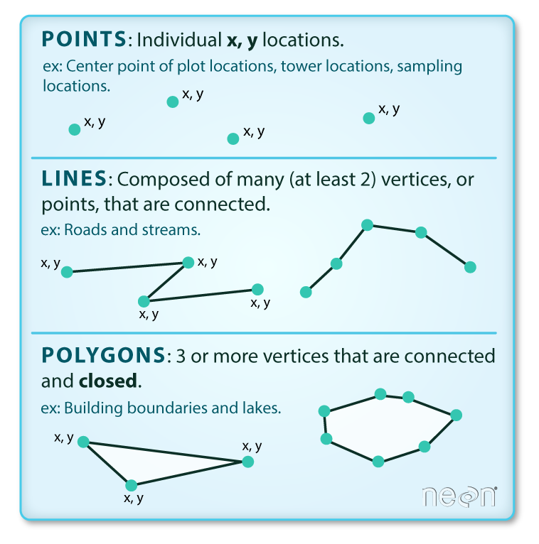
Source: National Ecological Observatory Network (NEON) http://datacarpentry.org/r-spatial-data-management-intro/images/dc-spatial-vector/pnt_line_poly.png

Points: Each individual point is define by a single x, y coordinate. There can be many points in a vector point file. Examples of point data include: sampling locations, the location of individual trees or the location of plots.
Lines: Lines are composed of many (at least 2) vertices that are connected. For instance, a road or a stream may be represented by a line. This line is composed of a series of segments, each “bend” in the road or stream represents a vertex that has defined x, y location.
Polygons: A polygon consists of 3 or more vertices that are connected and “closed”. Occasionally, a polygon can have a hole (or more than one) in the middle of it (like a doughnut), this is something to be aware of but not an issue we will deal with in this tutorial series. Objects often represented by polygons include: outlines of plot boundaries, lakes, oceans and states or country boundaries.

Some vector data formats can also include multipolygons (include several polygons) such as GeoJSON data format.

Shapefile

The most ubiquitous vector format is the ESRI shapefile. Geospatial Software company ESRI released the shapefile format specification as an open format in 1998. It was initially developed for their ArcView software but it became quickly an unofficial GIS standard.

Let’s take an example (downloaded from http://www.mapcruzin.com/free-norway-arcgis-maps-shapefiles.htm).

ls Norway_places

A-README.TXT  places.dbf  places.prj  places.shp  places.shx

When working with shapefiles, it is important to remember that a shapefile consists of 3 (or more) files:

.shp: the file that contains the geometry for all features.
.shx: the file that indexes the geometry.
.dbf: the file that stores feature attributes in a tabular format.

These files need to have the same name and to be stored in the same directory (folder) to open properly in a GIS, R or Python tool.

Sometimes, a shapefile will have other associated files including:

.prj: the file that contains information on projection format including the coordinate system and projection information. It is a plain text file describing the projection using well-known text (WKT) format.
.sbn and .sbx: the files that are a spatial index of the features.
.shp.xml: the file that is the geospatial metadata in XML format, (e.g. ISO 19115 or XML format).

Examine shapefile with python

from osgeo import ogr
shapedata = ogr.Open('Norway_places')

Type shapedata. and press TAB to see what you can do.

shapedata.CopyLayer            shapedata.Reference            shapedata.__len__
shapedata.CreateLayer          shapedata.Release              shapedata.__module__
shapedata.DeleteLayer          shapedata.ReleaseResultSet     shapedata.__new__
shapedata.Dereference          shapedata.TestCapability       shapedata.__reduce__
shapedata.Destroy              shapedata.__class__            shapedata.__reduce_ex__
shapedata.ExecuteSQL           shapedata.__del__              shapedata.__repr__
shapedata.GetDriver            shapedata.__delattr__          shapedata.__setattr__
shapedata.GetLayer             shapedata.__dict__             shapedata.__str__
shapedata.GetLayerByIndex      shapedata.__doc__              shapedata.__swig_destroy__
shapedata.GetLayerByName       shapedata.__getattr__          shapedata.__swig_getmethods__
shapedata.GetLayerCount        shapedata.__getattribute__     shapedata.__swig_setmethods__
shapedata.GetName              shapedata.__getitem__          shapedata.__weakref__
shapedata.GetRefCount          shapedata.__hash__             shapedata.name
shapedata.GetSummaryRefCount   shapedata.__init__             shapedata.this

For instance, to get the number of layers:

shapedata.GetLayerCount()

Data Tip:

A shapefile will only contain one type of vector data: points, lines or polygons.

Then get the first layer and all the points from this layer, with feature “NAME” and the coordinates of each location:

layer = shapedata.GetLayer()
places_norway = []
for i in range(layer.GetFeatureCount()):
    feature = layer.GetFeature(i)
    name = feature.GetField("NAME")
    geometry = feature.GetGeometryRef()
    places_norway.append([i,name,geometry.GetGeometryName(), geometry.Centroid().ExportToWkt()])

print(places_norway[0:10])

[[0, 'Gol', 'POINT', 'POINT (8.9436636 60.7016106)'], [1, 'Halhjem', 'POINT', 'POINT (5.4263602 60.1455207)'], [2, 'Tromsø', 'POINT', 'POINT (18.9517967 69.6669861)'], [3, 'Oslo', 'POINT', 'POINT (10.7391223 59.913263)'], [4, 'Narvik', 'POINT', 'POINT (17.426652 68.4396792)'], [5, 'Bergen', 'POINT', 'POINT (5.3289029 60.3934769)'], [6, 'Hamna', 'POINT', 'POINT (18.9827839 69.7031209)'], [7, 'Stakkevollan', 'POINT', 'POINT (19.0031056 69.6937324)'], [8, 'Storslett', 'POINT', 'POINT (21.0301562 69.7694272)'], [9, 'Kvaløysletta', 'POINT', 'POINT (18.8708572 69.6953085)']]

Source: http://www.mapcruzin.com/free-norway-arcgis-maps-shapefiles.htm

To get the coordinates of each location in a readable manner, we exported it to WKT (Well-Known Text) format which is now part of ISO/IEC 13249-3:2016 standard. Well-known text (WKT) is a text markup language for representing vector geometry objects on a map, spatial reference systems of spatial objects and transformations between spatial reference systems. We won’t discuss more about this format in this lesson and use it only for printing information from our shapefile.

In our previous example, we could call geometry.GetPoint() directly and get the very same information because our shapefile contains points only. Using the method Centroid() with polygons or lines would return a point only representing the centroids of the polygons or lines.

Shapefile with Points

We can then plot these locations on a map; as there were too many locations, we only plot locations of type city:

%matplotlib inline
from osgeo import ogr
from mpl_toolkits.basemap import Basemap
import matplotlib.pyplot as plt

fig = plt.figure(figsize=[12,15])  # a new figure window
ax = fig.add_subplot(1, 1, 1)  # specify (nrows, ncols, axnum)
ax.set_title('Cities in Norway', fontsize=14)

map = Basemap(llcrnrlon=-1.0,urcrnrlon=40.,llcrnrlat=55.,urcrnrlat=75.,
             resolution='i', projection='lcc', lat_1=65., lon_0=5.)

map.drawmapboundary(fill_color='aqua')
map.fillcontinents(color='#ffe2ab',lake_color='aqua')
map.drawcoastlines()

shapedata = ogr.Open('Norway_places')
layer = shapedata.GetLayer()
for i in range(layer.GetFeatureCount()):
    feature = layer.GetFeature(i)
    name = feature.GetField("NAME")
    type = feature.GetField("TYPE")
    if type == 'city':
        geometry = feature.GetGeometryRef()
        lon = geometry.GetPoint()[0]
        lat = geometry.GetPoint()[1]
        x,y = map(lon,lat)
        map.plot(x, y, marker=marker, color='red', markersize=8, markeredgewidth=2)
        ax.annotate(name, (x, y), color='blue', fontsize=14)

plt.show()

vector plot

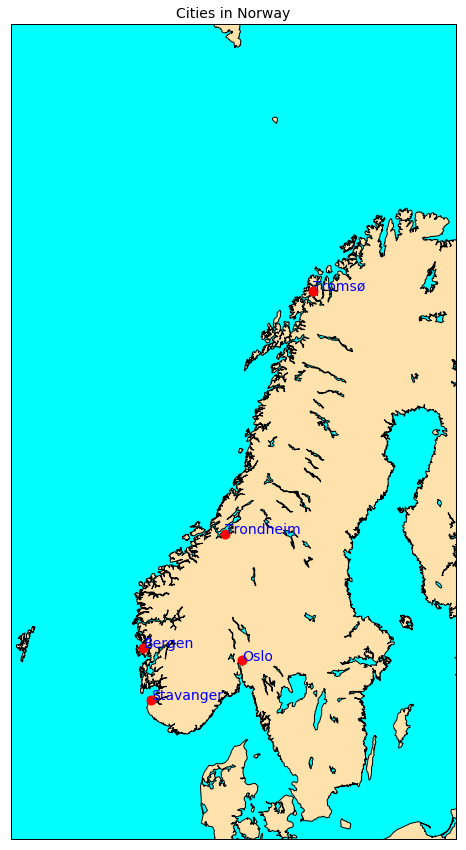
We do not explain here in details how we made this plot because this the purpose of the next lesson!

Shapefile with linestring

A shapefile with lines is very similar to a shapefile with points because each linestring is made of a set of points:

%matplotlib inline
shapedata = ogr.Open('Norway_railways')
nblayer = shapedata.GetLayerCount()
print("Number of layers: ", nblayer)
layer = shapedata.GetLayer()
railways_norway = []
for i in range(layer.GetFeatureCount()):
    feature = layer.GetFeature(i)
    name = feature.GetField("NAME")
    geometry = feature.GetGeometryRef()
    railways_norway.append([i,name,geometry.GetGeometryName(), geometry.GetPoints()])

print(railways_norway[0:10])

To visualize it:

vector plot

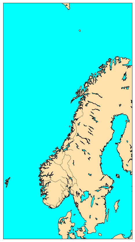
%matplotlib inline
from mpl_toolkits.basemap import Basemap
import matplotlib.pyplot as plt

fig = plt.figure(figsize=[12,15])  # a new figure window
ax = fig.add_subplot(1, 1, 1)  # specify (nrows, ncols, axnum)

map = Basemap(llcrnrlon=-1.0,urcrnrlon=40.,llcrnrlat=55.,urcrnrlat=75.,
             resolution='i', projection='lcc', lat_1=65., lon_0=5.)

map.drawmapboundary(fill_color='aqua')
map.fillcontinents(color='#ffe2ab',lake_color='aqua')
map.drawcoastlines()

norway_roads= map.readshapefile('Norway_roads/roads', 'roads')

plt.show()

Filter by attributes

 In the preceding example, we extracted all the locations from `Norway_places` and then made a plot for big cities only. 
 For this selection, we used a simple `if` statement. In this exercise, we show how to better filter by attributes.

 Use the preceding example to access information from `Norway_roads` but only for `Stolmakergata`. For instance, 
 use SetAttributeFilter and GetNexFeature to pick-up `stolmakergata` only.

Solution

We used SetAttributeFilter and GetNexFeature to select stolmakergata:

layer = shapedata.GetLayer()
layer.SetAttributeFilter("NAME = 'Stolmakergata'")
detail = layer.GetNextFeature()
geometry = detail.GetGeometryRef()
print("Type of geometry: ", geometry.GetGeometryName())
# go through each points of the line.
print(geometry.GetPointCount())
for i in range(geometry.GetPointCount()):
    xy = geometry.GetPoint(i)
    print(xy)

Shapefile with polygons

The image below shows a plot of a shapefile containing polygons:

vector plot

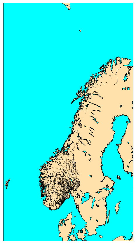
  The python code to make this plot is given below for information only. Plotting of shapefiles
  will be discussed in the next lesson.

%matplotlib inline
from mpl_toolkits.basemap import Basemap
import matplotlib.pyplot as plt
 
fig = plt.figure(figsize=[12,15])  # a new figure window
ax = fig.add_subplot(1, 1, 1)      # specify (nrows, ncols, axnum)
 
map = Basemap(llcrnrlon=-1.0,urcrnrlon=40.,llcrnrlat=55.,urcrnrlat=75.,
              resolution='i', projection='lcc', lat_1=65., lon_0=5.)
 
map.drawmapboundary(fill_color='aqua')
map.fillcontinents(color='#ffe2ab',lake_color='aqua')
map.drawcoastlines()

norway_natural= map.readshapefile('Norway_natural/natural', 'natural')
 
plt.show()

Explore Shapefile with polygons

 Use the preceding example to access information from `Norway_natural`. 
 You have to dig one level deeper and access the geometry contained within the polygon geometry. 
 The reason is that a polygon can have 'holes'. So the first polygon is what we call the outer rings
 and the other polygons are 'holes'
 Then the polygon information is stored as a line (set of points) so you can access each point
 of the polygon.

Solution

There is not one solution to this question but here is one way to do it:

layer = shapedata.GetLayer()
layer.SetAttributeFilter("NAME = 'Grasdalsvatnet'")
detail = layer.GetNextFeature()
geometry = detail.GetGeometryRef()
print("Type of geometry: ", geometry.GetGeometryName())
print("Number of 'rings': ", geometry.GetGeometryCount())
# Get the coordinates of the whole line                   
line = geometry.GetGeometryRef(0)
# all points in the line
print(line.GetPointCount())
for i in range(line.GetPointCount()):
    xy = line.GetPoint(i)
    print(xy)

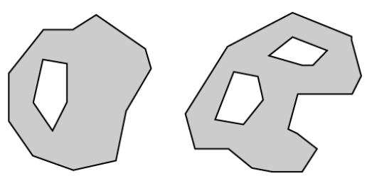
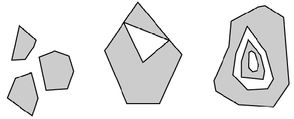
polygons versus multi-polygons:

polygons can have ‘holes’ as shown on the figure below:

but we can also have multi-polygons; and some of them with holes too!

GeoJSON

GeoJSON is an open standard format designed for representing simple geographical features, along with their non-spatial attributes, based on JavaScript Object Notation. For the full specifications of this standard, refer to RFC 7946.

This section is based on the GeoJSON documentation provided by Tom MacWright.

Handling GeoJSON in python is very similar to handling shapefiles and we can for instance use the same gdal ogr python package. However, before using python, let’s look at a simple GeoJSON file.

You can use your favourite editor to inspect the content of a simple GeoJSON file as it is a “text” file. It has some advantages (portable and readable on any machines) but as you will see when working with GeoJSON files, they can become very quickly too big compared to any binary counterpart.

Let’s look at

{
  "type": "FeatureCollection",
  "features": [
    {
      "type": "Feature",
      "geometry": {
        "type": "Point",
        "coordinates": [-118.17, 34.03]
      },
      "properties": {
        "name": "East Los Angeles CA",
        "country.etc": "CA",
        "pop": " 125121",
        "capital": "0"
      }
    }
  ]
}

GeoJSON supports the following geometry types:

Point,
LineString,
Polygon,
MultiPoint,
MultiLineString,
MultiPolygon.

Geometric objects with additional properties are Feature objects. Sets of features are contained by FeatureCollection objects.

To read the preceding file la_city.geoson in python, we can use gdal ogr and it is very similar to what we did when reading shapefiles:

from osgeo import ogr
la = ogr.Open('la_city.geojson')
nblayer = la.GetLayerCount()
print("Number of layers: ", nblayer)
layer = la.GetLayer()
cities_us = []
for i in range(layer.GetFeatureCount()):
    feature = layer.GetFeature(i)
    name = feature.GetField("NAME")
    geometry = feature.GetGeometryRef()
    cities_us.append([i,name,geometry.GetGeometryName(), geometry.GetPoints()])

print(cities_us)

It can of course become cumbersome with complex GeoJSON file containing MultiPolygons, MultiLineStrings, etc. but the principle remains the same. Let’s take another example:

Source: Grensedata Norge WGS84 Adm enheter geoJSON downloaded from kartverket; registration is free for open data access

from osgeo import ogr
shapedata = ogr.Open('no-all-all.geojson')
nblayer = shapedata.GetLayerCount()
print("Number of layers: ", nblayer)
layer = shapedata.GetLayer()
county_norway = []
for i in range(layer.GetFeatureCount()):
    feature = layer.GetFeature(i)
    name = feature.GetField("NAVN")
    geometry = feature.GetGeometryRef()
    county_norway.append([i,name,geometry.GetGeometryName(), geometry.Centroid().GetPoint()])
        
print(county_norway[0:10])

We will see more about GeoJSON when we discuss interctive visualization and publishing on the web.

Key Points

raster formats: GeoTIFF, netCDF, HDF data formats

vector formats: shapefile, GeoJSON data format

previous episode

Working with Spatio-temporal data in Python

next episode

Data Formats in Environmental Sciences

Overview

Types of Spatial Data

raster data formats

netCDF

Check a netCDF file?

netCDF and python?

Creating netCDF files

Create an empty netCDF4 dataset and store it on disk

Dimensions

Variables

Writing and Retrieving Data

Writing Data

Understand netCDF file

Solution

Retrieve Data

lats vs. lats[:]?

Solution

Types of netCDF files?

CF conventions?

HDF

Check an HDF file?

HDF data files and python?

Quick visualization with Python

Types of HDF files?

EOS Conventions?

HDF4 or HDF5?

Solution

Quick plot with imshow

Solution

GeoTIFF

vector data formats

Shapefile

Examine shapefile with python

Data Tip:

Shapefile with Points

Shapefile with linestring

Filter by attributes

Solution

Shapefile with polygons

Explore Shapefile with polygons

Solution

polygons versus multi-polygons:

GeoJSON

Key Points

previous episode

next episode