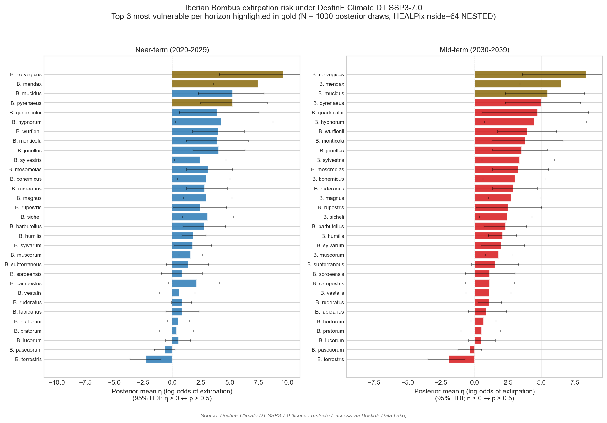
08 — Tier-2 projection figures (HEALPix nside=64)

Produces:

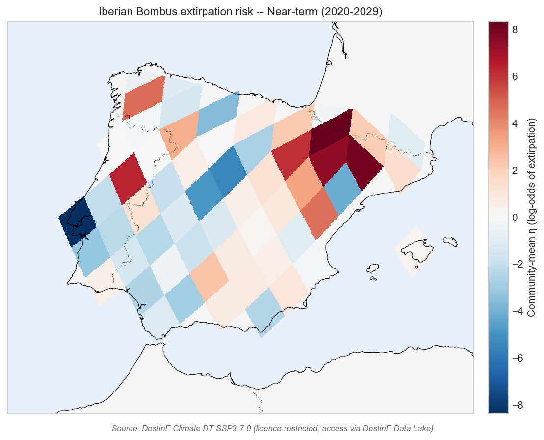
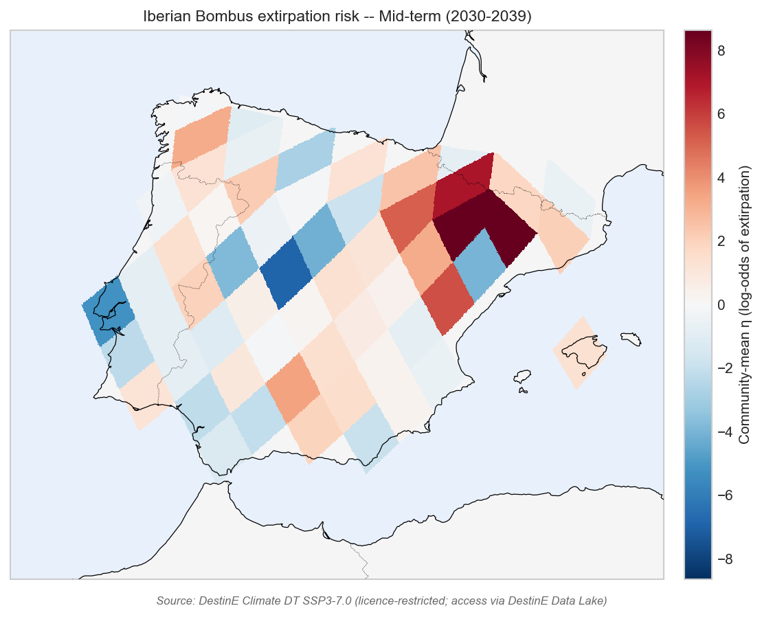
figures/projection_species_rank.png — two-panel ranked bar chart (near-term left, mid-term right) of per-species posterior-mean η (GLMM linear predictor / log-odds of extirpation) with 95 % HDI error bars; top-3 species per horizon highlighted in gold. η is reported instead of p = expit(η) because future predictors under SSP3-7.0 lie 5–10× outside the Tier-1 training distribution where logit saturation makes p uninterpretable.
figures/projection_risk_map_2020_2029.png — Iberia HEALPix nside=64 risk map of community-mean η, RdBu_r diverging colormap centred on η = 0 (= moderate-risk threshold p = 0.5).
figures/projection_risk_map_2030_2039.png — same, mid-term.
figures/projection_summary.png — combined panel for the Jupyter Book / nanopub Outcome draft (rank chart + the more impactful map).

Per DOMAIN.md: HEALPix is always NESTED, and we use healpix-geo (NOT healpy) for the cell→lat/lon mapping, since healpy is not geo-aware (cosmology-first, no CRS handling) and accumulates small biases over decadal timeseries.

import json
from pathlib import Path

import cartopy.crs as ccrs
import cartopy.feature as cfeature
import matplotlib.pyplot as plt
import numpy as np
import xarray as xr
import healpix_plot
from healpix_plot import HealpixGrid
# healpix_geo.nested.vertices is the canonical way to get the 4 corners
# of each HEALPix cell on a chosen ellipsoid (sphere | WGS84). Used for
# the native-polygon rendering in the projection-comparison figure.
from healpix_geo.nested import vertices as hp_vertices
from matplotlib.collections import PolyCollection

plt.style.use("seaborn-v0_8-whitegrid")

ROOT = Path("..").resolve()
HPORT = ROOT / "healpix_port"
OUT_DIR = HPORT / "outputs_iberia"
RESULTS_DIR = ROOT / "results"
PRECOMP = ROOT / "data" / "precomputed"
FIG_DIR = ROOT / "figures"
FIG_DIR.mkdir(parents=True, exist_ok=True)

# Iberia nside=64 cells (depth=6, NESTED).
DEPTH = 6
IBERIA_PIX_64 = np.load(PRECOMP / "iberia_pix_nside64_nested.npy").astype(np.uint64)
N_64 = len(IBERIA_PIX_64)
print(f"Iberia HEALPix nside=64 cells: {N_64}")

Load projection summary + per-cell rasters¶

with open(RESULTS_DIR / "projection_headline.json") as f:
    summary = json.load(f)

HORIZONS = ["2020_2029", "2030_2039"]
HORIZON_TITLES = {
    "2020_2029": "Near-term (2020-2029)",
    "2030_2039": "Mid-term (2030-2039)",
}

per_cell = {}
for h in HORIZONS:
    p = RESULTS_DIR / f"projection_{h}.nc"
    if p.exists():
        ds_p = xr.open_dataset(p)
        per_cell[h] = ds_p["community_mean_eta"].values.astype(float)
        print(f"  loaded {p.name}: shape {per_cell[h].shape}")
    else:
        print(f"  [missing] {p}")

HEALPix plotting via `healpix_plot` (EOPF-DGGS canonical)¶

We use healpix_plot.plot() — the EOPF-DGGS-canonical HEALPix + cartopy plotting bridge (per DOMAIN.md: *"replaces ad-hoc ang2pix

pcolormesh bridges"*). Internally it:

Resamples the 120 sparse nside=64 NESTED cells onto a dense regular lon/lat grid (nearest-neighbour by default) at the requested view extent.
Renders the resampled raster cleanly in any cartopy projection.

This replaces our previous manual PolyCollection of cell-vertex polygons, which had two visual artefacts: (a) diamond-oriented polygons that — although technically correct HEALPix geometry for the equatorial belt — looked geometrically unfamiliar; (b) straight-edge approximation in PlateCarree caused micro-overlap at sub-pixel boundaries.

HPX_GRID = HealpixGrid(level=DEPTH, indexing_scheme="nested", ellipsoid="WGS84")
print(f"HealpixGrid: level={DEPTH} (nside={2**DEPTH}), NESTED, WGS84")

# Pre-compute the on-WGS84 cell vertices once. Used by the native-polygon
# rendering in the projection-comparison figure (lets cartopy reproject
# the WGS84 vertices through any target CRS).
_lon_v, _lat_v = hp_vertices(IBERIA_PIX_64, DEPTH, ellipsoid="WGS84")
_lon_v = np.where(_lon_v > 180.0, _lon_v - 360.0, _lon_v)
WGS84_POLY_XY = np.stack([_lon_v, _lat_v], axis=-1)   # (N_64, 4, 2)
print(f"WGS84 cell-vertex polygon array: shape={WGS84_POLY_XY.shape}")

Helper: ranked bar chart on a given matplotlib axis¶

GOLD = "#d4a017"
DARK_GOLD = "#8a6a0c"
TEAL = "#2c7bb6"
ORANGE = "#d7191c"
DATA_FOOTER = (
    "Source: DestinE Climate DT SSP3-7.0 "
    "(licence-restricted; access via DestinE Data Lake)"
)


def _plot_rank(ax, records, title, color, order_species=None,
               highlight_species=None):
    """Horizontal bar chart of per-species posterior-mean η (linear
    predictor / log-odds of extirpation under SSP3-7.0). η is reported
    instead of p = expit(η) because future predictors lie 5–10× outside
    the Tier-1 training distribution where logit saturation makes p
    uninterpretable. See 05_outcome.md § Limitations.

    If `order_species` is given, the species are reordered to match
    (any species not present in `records` are dropped); otherwise the
    input order of `records` is preserved.

    `highlight_species` (set or list) controls which bars are drawn
    in dark gold; defaults to the top-3 species *in the displayed
    order*.
    """
    by_name = {r["species"]: r for r in records}
    if order_species is not None:
        species = [sp for sp in order_species if sp in by_name]
    else:
        species = [r["species"] for r in records]

    means = np.array([by_name[sp]["post_mean_eta"] for sp in species])
    los = np.array([by_name[sp]["eta_hdi95_low"] for sp in species])
    his = np.array([by_name[sp]["eta_hdi95_high"] for sp in species])

    y = np.arange(len(species))
    err = np.vstack([means - los, his - means])

    if highlight_species is None:
        # Highlight the top-3 by posterior-mean within this panel
        top3 = set(sorted(species, key=lambda s: -by_name[s]["post_mean_eta"])[:3])
    else:
        top3 = set(highlight_species)
    bar_colors = [DARK_GOLD if sp in top3 else color for sp in species]

    ax.barh(y, means, color=bar_colors, alpha=0.85, edgecolor="white")
    ax.errorbar(means, y, xerr=err, fmt="none", ecolor="black",
                elinewidth=0.8, capsize=2, alpha=0.5)
    # Reference line at η = 0 (= log-odds 0 ↔ p = 0.5, the moderate-risk
    # threshold). Species with η > 0 across most cells are projected to
    # be more likely than not to be extirpated under SSP3-7.0.
    ax.axvline(0, color="black", linewidth=0.6, linestyle="--", alpha=0.4)
    ax.set_yticks(y)
    ax.set_yticklabels([f"B. {sp}" for sp in species], fontsize=8)
    ax.invert_yaxis()
    ax.set_xlabel("Posterior-mean η (log-odds of extirpation)\n(95% HDI; η > 0 ↔ p > 0.5)")
    ax.set_title(title, fontsize=11)
    span = max(abs(means.min()), abs(means.max()))
    ax.set_xlim(-span * 1.15, span * 1.15)
    ax.grid(axis="x", linewidth=0.3, alpha=0.5)

Helper: HEALPix-cell polygon map on a given cartopy axis¶

def _draw_healpix_map(ax, raster_per_cell, title):
    """Draw the Iberia raster via `healpix_plot.plot` (EOPF-DGGS canonical),
    in **ETRS89 / LAEA Europe (EPSG:3035)** — the canonical European
    biodiversity reporting CRS (EEA / Natura 2000 / EUNIS / INSPIRE) and
    an equal-area projection that respects HEALPix's native equal-area
    pixelisation. PlateCarree would distort cells visually relative to
    their on-sphere areas — not faithful to the substrate.

    Diverging colormap centred on η = 0 (the moderate-risk threshold:
    log-odds 0 ↔ p = 0.5). Red cells = high projected extirpation
    tendency; blue = low; white ≈ moderate. We plot η rather than
    p = expit(η) because future predictors lie far outside training
    distribution and expit() saturates uninformatively.
    """
    # The caller passes an axis already configured with EPSG:3035
    # (LAEA Europe). We declare the extent in PlateCarree (lon/lat)
    # — cartopy does the projection internally.
    pc = ccrs.PlateCarree()
    ax.set_extent([-10.5, 4.5, 35.0, 44.5], crs=pc)
    ax.add_feature(cfeature.LAND, facecolor="#f5f5f5", zorder=0)
    ax.add_feature(cfeature.OCEAN, facecolor="#e8f0fb", zorder=0)

    valid = np.isfinite(raster_per_cell)
    if valid.sum() == 0:
        ax.set_title(title + " (no data)", fontsize=11)
        return None

    span = max(0.5, float(np.nanpercentile(np.abs(raster_per_cell), 98)))

    # `healpix_plot.plot` resamples the 120 sparse NESTED cells onto a
    # regular grid at the requested `view` extent and plots in cartopy.
    # Returns an AxesImage we can attach a colorbar to. shape=600 is
    # ample for a 14°×9° view at nside=64 (~92 km cells).
    img = healpix_plot.plot(
        cell_ids=IBERIA_PIX_64.astype(np.uint64),
        data=raster_per_cell.astype(np.float64),
        healpix_grid=HPX_GRID,
        sampling_grid={"shape": 600},
        view=(-10.5, 4.5, 35.0, 44.5),
        interpolation="nearest",
        background_value=np.nan,
        ax=ax,
        cmap="RdBu_r",
        vmin=-span,
        vmax=+span,
        title=None,    # we set the title below to keep style consistent
    )
    # Re-overlay coastlines + borders ON TOP of the resampled raster
    # (healpix_plot draws into ax, which clobbers our zordered features).
    ax.add_feature(cfeature.COASTLINE, linewidth=0.6, zorder=3)
    ax.add_feature(cfeature.BORDERS, linewidth=0.4, linestyle=":", zorder=3)
    ax.set_title(title, fontsize=11)
    return img

Figure 1 — species-rank chart (two panels)¶

fig, axes = plt.subplots(1, 2, figsize=(13, 9), sharey=False)
records_near = summary["horizons"]["2020_2029"]["species_ranked"]
records_mid = summary["horizons"]["2030_2039"]["species_ranked"]

# Sort *both* panels by mid-term posterior-mean, so the eye can track
# rank shifts across horizons. Highlight the top-3 most-vulnerable in
# each horizon (per its own ranking) in dark gold.
def _top3_species(records):
    return [r["species"] for r in
            sorted(records, key=lambda r: -r["post_mean_eta"])[:3]]


mid_order = [
    r["species"] for r in
    sorted(records_mid, key=lambda r: -r["post_mean_eta"])
]
top3_near = set(_top3_species(records_near))
top3_mid = set(_top3_species(records_mid))

_plot_rank(axes[0], records_near, HORIZON_TITLES["2020_2029"], TEAL,
           order_species=mid_order, highlight_species=top3_near)
_plot_rank(axes[1], records_mid, HORIZON_TITLES["2030_2039"], ORANGE,
           order_species=mid_order, highlight_species=top3_mid)
fig.suptitle(
    "Iberian Bombus extirpation risk under DestinE Climate DT SSP3-7.0\n"
    f"Top-3 most-vulnerable per horizon highlighted in gold "
    f"(N = {summary['method']['n_posterior_draws']} posterior draws, "
    f"HEALPix nside=64 NESTED)",
    fontsize=12,
)
fig.text(
    0.5, 0.005, DATA_FOOTER,
    ha="center", va="bottom", fontsize=8, color="dimgray", style="italic",
)
fig.tight_layout(rect=[0, 0.03, 1, 0.95])
out = FIG_DIR / "projection_species_rank.png"
fig.savefig(out, dpi=150, bbox_inches="tight")
plt.show()
print(f"Saved {out}")

Native-polygon HEALPix-on-WGS84 helper¶

Renders the 110 nside=64 cells as their actual on-WGS84 quadrilateral polygons (vertices from healpix_geo.nested.vertices(..., ellipsoid="WGS84")). Lets cartopy reproject the polygon edges into whatever the axis CRS is, so the same physical cells can be visualised in PlateCarree (lon/lat direct), LAEA Europe, etc. NO RESAMPLING — preserves cell-boundary geometry exactly as defined by the WGS84 ellipsoid + HEALPix indexing.

(Contrast with _draw_healpix_map above which uses healpix_plot.plot() to resample onto a regular grid in the axis CRS. That gives a clean continuous raster but loses cell boundaries.)

def _draw_healpix_polygons_native(ax, raster_per_cell, title):
    """Render HEALPix cells as their native WGS84-ellipsoid polygons,
    reprojected by cartopy into the axis's CRS. Diverging RdBu_r
    centred on η=0; same colour scaling as `_draw_healpix_map`.
    """
    pc = ccrs.PlateCarree()
    ax.set_extent([-10.5, 4.5, 35.0, 44.5], crs=pc)
    ax.add_feature(cfeature.LAND, facecolor="#f5f5f5", zorder=0)
    ax.add_feature(cfeature.OCEAN, facecolor="#e8f0fb", zorder=0)

    valid = np.isfinite(raster_per_cell)
    if valid.sum() == 0:
        ax.set_title(title + " (no data)", fontsize=11)
        return None

    span = max(0.5, float(np.nanpercentile(np.abs(raster_per_cell), 98)))

    polys = WGS84_POLY_XY[valid]
    vals = raster_per_cell[valid]
    pcoll = PolyCollection(
        polys,
        array=vals,
        cmap="RdBu_r",
        norm=plt.Normalize(vmin=-span, vmax=+span),
        edgecolors="black",
        linewidths=0.15,
        transform=pc,           # vertices are WGS84 lon/lat → reproject via PlateCarree CRS
        zorder=1,
    )
    ax.add_collection(pcoll)
    # Coastlines on top of the polygons.
    ax.add_feature(cfeature.COASTLINE, linewidth=0.6, zorder=3)
    ax.add_feature(cfeature.BORDERS, linewidth=0.4, linestyle=":", zorder=3)
    ax.set_title(title, fontsize=11)
    return pcoll

Figures 2 + 3 — per-cell community-mean risk maps¶


def _plot_map(horizon: str, raster: np.ndarray) -> Path:
    # ETRS89 / LAEA Europe (EPSG:3035) — equal-area, canonical EU
    # biodiversity reporting CRS. Faithful to HEALPix's equal-area
    # pixelisation.
    proj = ccrs.epsg(3035)
    fig = plt.figure(figsize=(7.5, 6))
    ax = plt.axes(projection=proj)
    pc = _draw_healpix_map(
        ax, raster,
        f"Iberian Bombus extirpation risk -- {HORIZON_TITLES[horizon]}",
    )
    if pc is not None:
        cbar = plt.colorbar(pc, ax=ax, orientation="vertical",
                            fraction=0.04, pad=0.03)
        cbar.set_label("Community-mean η (log-odds of extirpation)")
    fig.text(
        0.5, 0.01, DATA_FOOTER,
        ha="center", va="bottom", fontsize=8, color="dimgray", style="italic",
    )
    fig.tight_layout(rect=[0, 0.03, 1, 1])
    out = FIG_DIR / f"projection_risk_map_{horizon}.png"
    fig.savefig(out, dpi=150, bbox_inches="tight")
    plt.show()
    return out


for h in HORIZONS:
    if h not in per_cell:
        print(f"  [skip] {h}")
        continue
    out = _plot_map(h, per_cell[h])
    print(f"Saved {out}")

Option B nside=128 standalone risk maps (DestinE-resolution)¶

Same per-cell community-mean η as the nside=64 maps above, but at the full DestinE nside=128 resolution (~46 km cells, ~440 in Iberia). The GLMM is unchanged (calibrated at nside=64); the gain is in spatial detail of the climate predictors. Within each nside=64 parent the 4 children share the same per-species random effect but their TEI/PEI deltas vary because DestinE provides the finer climate.

HPX_GRID_128 = HealpixGrid(level=7, indexing_scheme="nested", ellipsoid="WGS84")

per_cell_128 = {}
for h in HORIZONS:
    p = RESULTS_DIR / f"projection_{h}_nside128.nc"
    if p.exists():
        ds_p128 = xr.open_dataset(p)
        per_cell_128[h] = ds_p128["community_mean_eta"].values.astype(float)
        print(f"  loaded {p.name}: shape {per_cell_128[h].shape}")
    else:
        print(f"  [missing] {p}")

# Pre-compute the nside=128 Iberian indices (same as 06's IBERIA_PIX_128).
IBERIA_PIX_128 = np.load(PRECOMP / "iberia_pix_nside128_nested.npy").astype(np.uint64)


def _plot_map_nside128(horizon: str, raster: np.ndarray) -> Path:
    proj = ccrs.epsg(3035)
    fig = plt.figure(figsize=(7.5, 6))
    ax = plt.axes(projection=proj)
    pc = ccrs.PlateCarree()
    ax.set_extent([-10.5, 4.5, 35.0, 44.5], crs=pc)
    ax.add_feature(cfeature.LAND, facecolor="#f5f5f5", zorder=0)
    ax.add_feature(cfeature.OCEAN, facecolor="#e8f0fb", zorder=0)

    valid = np.isfinite(raster)
    if valid.sum() == 0:
        ax.set_title(
            f"Iberian Bombus extirpation risk -- {HORIZON_TITLES[horizon]} "
            "(nside=128, no data)"
        )
        return None
    span = max(0.5, float(np.nanpercentile(np.abs(raster), 98)))

    img = healpix_plot.plot(
        cell_ids=IBERIA_PIX_128,
        data=raster.astype(np.float64),
        healpix_grid=HPX_GRID_128,
        sampling_grid={"shape": 800},
        view=(-10.5, 4.5, 35.0, 44.5),
        interpolation="nearest",
        background_value=np.nan,
        ax=ax,
        cmap="RdBu_r",
        vmin=-span,
        vmax=+span,
        title=None,
    )
    ax.add_feature(cfeature.COASTLINE, linewidth=0.6, zorder=3)
    ax.add_feature(cfeature.BORDERS, linewidth=0.4, linestyle=":", zorder=3)
    ax.set_title(
        f"Iberian Bombus extirpation risk -- {HORIZON_TITLES[horizon]} "
        "(Option B: nside=128, DestinE resolution)",
        fontsize=11,
    )
    if img is not None:
        cbar = plt.colorbar(img, ax=ax, orientation="vertical",
                            fraction=0.04, pad=0.03)
        cbar.set_label("Community-mean η (log-odds of extirpation)")
    fig.text(
        0.5, 0.01, DATA_FOOTER,
        ha="center", va="bottom", fontsize=8, color="dimgray", style="italic",
    )
    fig.tight_layout(rect=[0, 0.03, 1, 1])
    out = FIG_DIR / f"projection_risk_map_{horizon}_nside128.png"
    fig.savefig(out, dpi=150, bbox_inches="tight")
    plt.show()
    return out


for h in HORIZONS:
    if h not in per_cell_128:
        continue
    out = _plot_map_nside128(h, per_cell_128[h])
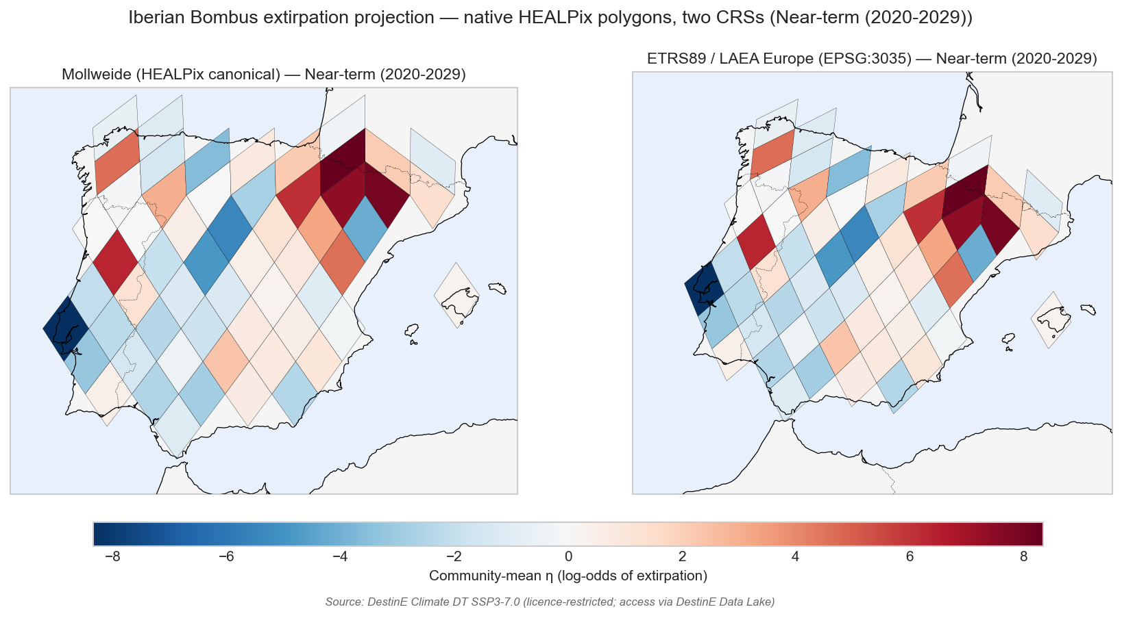
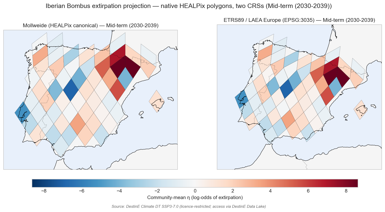
    print(f"Saved {out}")

Projection comparison — native HEALPix-on-WGS84 polygons in two CRSs¶

Same physical HEALPix cells (vertices computed on the WGS84 ellipsoid via healpix_geo.nested.vertices(..., ellipsoid="WGS84")), rendered as native polygons (no resampling), reprojected by cartopy into two different cartographic projections. Same colormap, same colorbar — only the cartographic CRS differs.

Left — Mollweide (HEALPix canonical): equal-area pseudocylindrical projection — the canonical HEALPix display (Górski et al. 2005). Faithful to HEALPix’s equal-area pixelisation. At Iberia scale the curvature is subtle; the “Mollweide character” is more visible at global scale (see the standalone Iberia map for the LAEA-only view).
Right — ETRS89 / LAEA Europe (EPSG:3035): same polygons, but cartopy reprojects each vertex through Europe’s canonical equal-area CRS (LAEA centred on lat 52° N, lon 10° E). Cells appear in their true relative areas. Canonical EEA / Natura 2000 / EUNIS / INSPIRE biodiversity reporting CRS.

Both projections are equal-area and both panels render via native polygon transformation (no rendering-method confound). Use this figure to answer “does projection choice affect cell shape / relative area at the regional scale?” — at Iberia size, both equal-area projections give nearly identical visual proportions, with subtle orientation differences (LAEA tilts Iberia toward Europe’s centre; Mollweide preserves north-up orientation at Iberia’s longitude).

def _plot_proj_comparison(horizon: str, raster: np.ndarray) -> Path:
    """Side-by-side same-data, two-projection comparison map.
    Both panels render the same WGS84-ellipsoid HEALPix polygons —
    only the cartopy projection differs (both equal-area)."""
    fig = plt.figure(figsize=(14, 6))
    ax_left = fig.add_subplot(1, 2, 1, projection=ccrs.Mollweide())
    ax_right = fig.add_subplot(1, 2, 2, projection=ccrs.epsg(3035))

    pc_left = _draw_healpix_polygons_native(
        ax_left, raster,
        f"Mollweide (HEALPix canonical) — {HORIZON_TITLES[horizon]}",
    )
    pc_right = _draw_healpix_polygons_native(
        ax_right, raster,
        f"ETRS89 / LAEA Europe (EPSG:3035) — {HORIZON_TITLES[horizon]}",
    )

    # Shared colorbar; both panels use the same RdBu_r mapping with
    # span computed from the raster, which is the same in both calls.
    if pc_right is not None:
        cbar = fig.colorbar(
            pc_right, ax=[ax_left, ax_right], orientation="horizontal",
            fraction=0.05, pad=0.06, aspect=40,
        )
        cbar.set_label("Community-mean η (log-odds of extirpation)")

    fig.suptitle(
        f"Iberian Bombus extirpation projection — native HEALPix polygons, "
        f"two CRSs ({HORIZON_TITLES[horizon]})",
        fontsize=13,
    )
    fig.text(
        0.5, 0.01, DATA_FOOTER,
        ha="center", va="bottom", fontsize=8, color="dimgray", style="italic",
    )
    out = FIG_DIR / f"projection_proj_comparison_{horizon}.png"
    fig.savefig(out, dpi=150, bbox_inches="tight")
    plt.show()
    return out


for h in HORIZONS:
    if h not in per_cell:
        continue
    out = _plot_proj_comparison(h, per_cell[h])
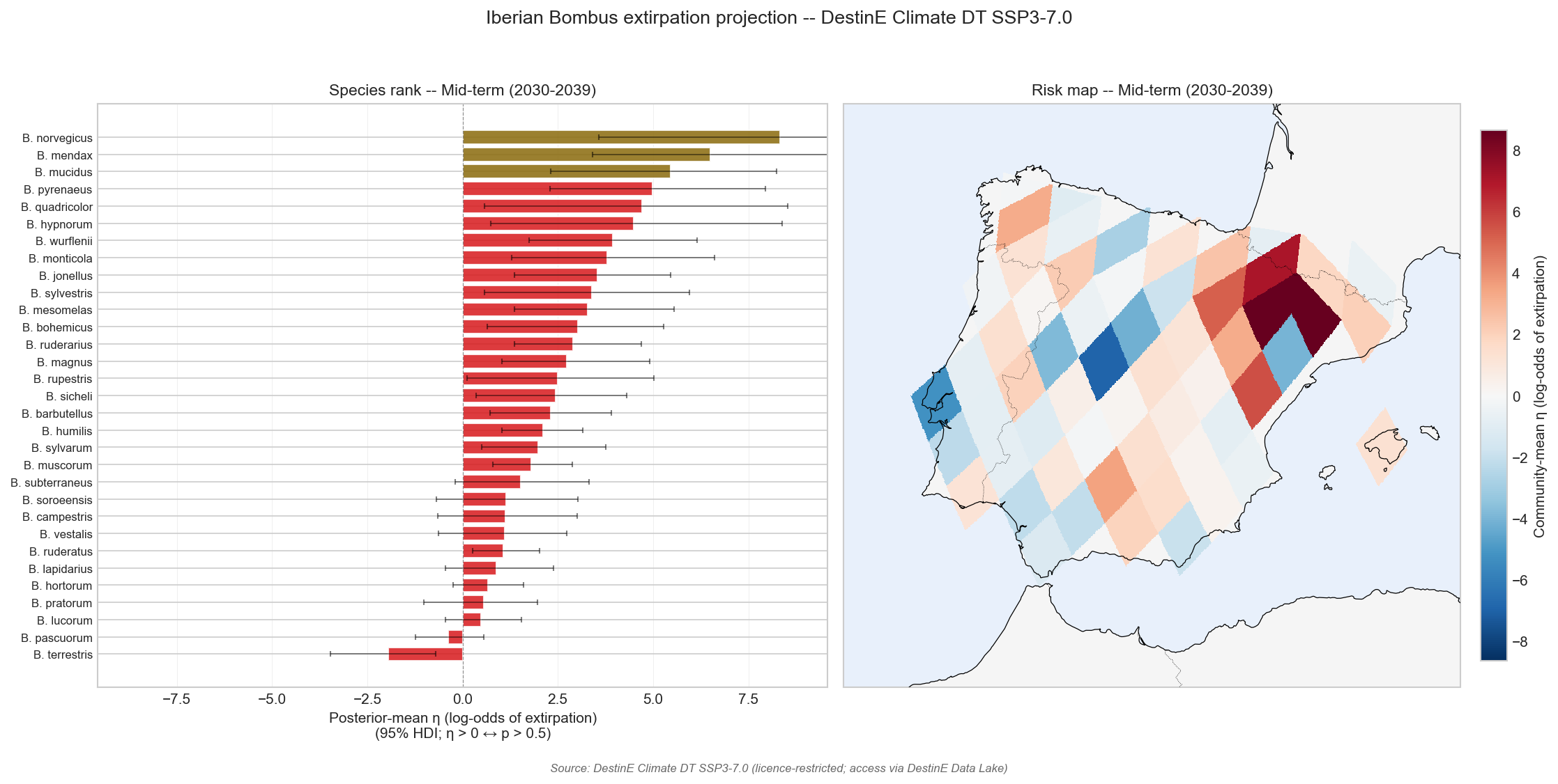
    print(f"Saved {out}")

Figure 4 — combined summary panel for the Jupyter Book¶

# The combined panel is the headline figure for the FORRT Outcome.
# Select the horizon with the higher posterior-mean community risk
# (median across cells) — this is more representative of the broad
# shift than the per-cell max (which is sensitive to the rare species
# with very few historical cells).
def _median_risk(h):
    if h not in per_cell:
        return -np.inf
    arr = per_cell[h]
    finite = arr[np.isfinite(arr)]
    return float(np.median(finite)) if finite.size else -np.inf


impactful = "2030_2039"
if per_cell:
    impactful = max(per_cell.keys(), key=_median_risk)
print(f"Combined panel uses {impactful} for the map "
      f"(median community risk = {_median_risk(impactful):.3f}).")

fig = plt.figure(figsize=(15, 7.5))
gs = fig.add_gridspec(1, 2, width_ratios=[1.1, 1.0])

ax_rank = fig.add_subplot(gs[0, 0])
records = summary["horizons"][impactful]["species_ranked"]
_plot_rank(
    ax_rank, records,
    f"Species rank -- {HORIZON_TITLES[impactful]}",
    ORANGE if impactful == "2030_2039" else TEAL,
)

if impactful in per_cell:
    ax_map = fig.add_subplot(gs[0, 1], projection=ccrs.epsg(3035))
    pc = _draw_healpix_map(
        ax_map, per_cell[impactful],
        f"Risk map -- {HORIZON_TITLES[impactful]}",
    )
    if pc is not None:
        plt.colorbar(
            pc, ax=ax_map, orientation="vertical",
            fraction=0.04, pad=0.03,
            label="Community-mean η (log-odds of extirpation)",
        )

fig.suptitle(
    "Iberian Bombus extirpation projection -- DestinE Climate DT SSP3-7.0",
    fontsize=13,
)
fig.text(
    0.5, 0.005, DATA_FOOTER,
    ha="center", va="bottom", fontsize=8, color="dimgray", style="italic",
)
fig.tight_layout(rect=[0, 0.03, 1, 0.95])
out = FIG_DIR / "projection_summary.png"
fig.savefig(out, dpi=150, bbox_inches="tight")
plt.show()
print(f"Saved {out}")

Tier-2 figures (committed; CI-renderable)¶

Tier-2 notebooks 05–08 require DestinE Climate DT credentials, so this chapter cannot execute on a generic GitHub Actions runner. The figures below are the committed PNGs from the local DestinE-platform run.