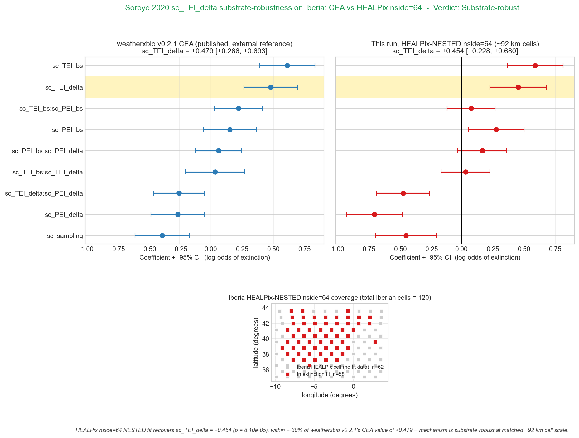
Phase C — substrate-robustness branch. Side-by-side forest plot
comparing weatherxbio v0.2.1 CEA published values (left, embedded
inline as a CSV string) vs this run’s HEALPix nside=64 fit
(right). The headline coefficient sc_TEI_delta is highlighted in
gold in both panels; the verdict (“Substrate-robust” or
“Substrate-divergent”) is annotated above the figure based on the
substrate-robustness JSON written by 03h_analysis_healpix.py.
Optional Iberia HEALPix coverage map at the bottom shows the nside=64 cells used in the fit.
Output: figures/main_result_healpix.png. Style: seaborn-v0_8-whitegrid,
150 dpi, plt.show() after fig.savefig() per the project conventions.
import io
import json
from pathlib import Path

import matplotlib.pyplot as plt
import numpy as np
import pandas as pd
import xarray as xr
plt.style.use("seaborn-v0_8-whitegrid")
ROOT = Path("..").resolve()
PORT = ROOT / "healpix_port"
OUT_DIR = PORT / "outputs_iberia"
RESULTS_DIR = ROOT / "results"
FIG_DIR = ROOT / "figures"
FIG_DIR.mkdir(parents=True, exist_ok=True)Load the HEALPix re-run posterior + headline JSON
hp_post = pd.read_csv(OUT_DIR / "posterior_vb_summary.csv", index_col=0)
print("HEALPix posterior (VB):")
print(hp_post.round(4).to_string())

with open(RESULTS_DIR / "headline_statistic_healpix.json") as f:
    headline = json.load(f)
verdict = headline["substrate_robustness"]["verdict"]
verdict_comment = headline["substrate_robustness"]["comment"]
all_pass = headline["substrate_robustness"]["all_three_pass"]
print(f"\nVerdict: {verdict}")
weatherxbio v0.2.1 CEA published posterior (verbatim)
Embedded inline (verbatim from
soroye_port/outputs_iberia/posterior_vb_summary.csv at tag v0.2.1)
so this comparison stays meaningful regardless of what the local
soroye_port/ re-run produces. This is the external reference for
the substrate-robustness test, NOT this repo’s local CEA rerun.
CEA_CSV = """\
,mean,sd,z,p_2sided
Intercept,-0.7400648781994158,0.1076178489098709,-6.876785641935793,6.121769757783113e-12
sc_sampling,-0.3875341930083687,0.11040852959191834,-3.510002301821574,0.0004481028148530797
sc_TEI_bs,0.6112635536304514,0.1129182331265557,5.41332906746215,6.186364887028617e-08
sc_TEI_delta,0.47922142481765523,0.10900153430642859,4.3964649476442474,1.100281192822905e-05
sc_TEI_bs:sc_TEI_delta,0.03464586746713759,0.12131364100510114,0.2855892147007669,0.7751927649919219
sc_PEI_bs,0.153608361852161,0.1085750812853235,1.4147662615927032,0.1571370392259941
sc_PEI_delta,-0.26270859409848013,0.10929945813422809,-2.403567214174602,0.016235981996329363
sc_PEI_bs:sc_PEI_delta,0.062442665853287935,0.09380392170626804,0.6656722311548673,0.5056206265192014
sc_TEI_bs:sc_PEI_bs,0.22153322565627676,0.09770397731566262,2.267392093369401,0.023366284065860166
sc_TEI_delta:sc_PEI_delta,-0.25309431271815575,0.1036799129619303,-2.441112318555747,0.014642100019127247
"""
cea_post = pd.read_csv(io.StringIO(CEA_CSV), index_col=0)
Side-by-side forest plot
Two top panels: weatherxbio v0.2.1 CEA published (left) vs this run’s
HEALPix nside=64 fit (right). Coefficients are ordered by the CEA
posterior mean (so panels are visually aligned). The sc_TEI_delta
row is highlighted in gold. Bottom panel: a small Iberia HEALPix
coverage map showing the nside=64 cells included in the fit.
def order_for_plot(df: pd.DataFrame) -> pd.DataFrame:
    return df.drop("Intercept", errors="ignore").copy()


cea = order_for_plot(cea_post)
hp = order_for_plot(hp_post)

order = cea.sort_values("mean", ascending=True).index.tolist()
cea = cea.reindex(order)
hp = hp.reindex(order)


def _plot_panel(ax, df, color, title):
    y = np.arange(len(df))
    ci = 1.96 * df["sd"]
    ax.errorbar(
        df["mean"], y, xerr=ci,
        fmt="o", color=color, ecolor=color,
        capsize=4, markersize=7, elinewidth=1.5,
    )
    ax.axvline(0, color="k", linewidth=0.5)
    if "sc_TEI_delta" in df.index:
        idx = df.index.tolist().index("sc_TEI_delta")
        ax.axhspan(idx - 0.5, idx + 0.5, facecolor="gold",
                   alpha=0.25, zorder=0)
    ax.set_yticks(y)
    ax.set_yticklabels(df.index)
    ax.set_xlabel("Coefficient +- 95% CI  (log-odds of extinction)")
    ax.set_title(title, fontsize=11)
    ax.grid(axis="x", linewidth=0.3, alpha=0.5)
Iberia HEALPix coverage map (cells included in the fit)
pa = xr.open_dataset(OUT_DIR / "presence_absence_healpix.nc")
iberia_lon = pa["lon"].values.astype(float)
iberia_lat = pa["lat"].values.astype(float)
n_cells_iberia = int(pa.sizes['cells'])

# Cells that ended up in the fit (extinction subset)
data_ext = pd.read_parquet(OUT_DIR / "dataGLMM_extinction.parquet")
fit_cell_idxs = sorted(data_ext["site"].unique().tolist())
fit_mask = np.zeros(n_cells_iberia, dtype=bool)
fit_mask[fit_cell_idxs] = True
print(f"\nCells in extinction fit: {fit_mask.sum()} / {n_cells_iberia}")
fig = plt.figure(figsize=(13.5, 9.0))
gs = fig.add_gridspec(
nrows=2, ncols=2,
height_ratios=[2.4, 1.0],
hspace=0.45, wspace=0.05,
)
ax_left = fig.add_subplot(gs[0, 0])
ax_right = fig.add_subplot(gs[0, 1], sharey=ax_left)
ax_map = fig.add_subplot(gs[1, :])
cea_tei = cea.loc["sc_TEI_delta"]
hp_tei = hp.loc["sc_TEI_delta"]
_plot_panel(
ax_left, cea, color="#2c7bb6",
title=(
"weatherxbio v0.2.1 CEA (published, external reference)\n"
f"sc_TEI_delta = {cea_tei['mean']:+.3f} "
f"[{cea_tei['mean'] - 1.96 * cea_tei['sd']:+.3f}, "
f"{cea_tei['mean'] + 1.96 * cea_tei['sd']:+.3f}]"
),
)
_plot_panel(
ax_right, hp, color="#d7191c",
title=(
"This run, HEALPix-NESTED nside=64 (~92 km cells)\n"
f"sc_TEI_delta = {hp_tei['mean']:+.3f} "
f"[{hp_tei['mean'] - 1.96 * hp_tei['sd']:+.3f}, "
f"{hp_tei['mean'] + 1.96 * hp_tei['sd']:+.3f}]"
),
)
# Match x-limits between the two top panels.
xmin = min(ax_left.get_xlim()[0], ax_right.get_xlim()[0])
xmax = max(ax_left.get_xlim()[1], ax_right.get_xlim()[1])
ax_left.set_xlim(xmin, xmax)
ax_right.set_xlim(xmin, xmax)
plt.setp(ax_right.get_yticklabels(), visible=False)HEALPix Iberia coverage map (bottom)
ax_map.scatter(
    iberia_lon[~fit_mask], iberia_lat[~fit_mask],
    s=26, c="#cccccc", marker="s",
    label=f"Iberia HEALPix cell (no fit data)  n={(~fit_mask).sum()}",
    edgecolor="white", linewidth=0.4,
)
ax_map.scatter(
    iberia_lon[fit_mask], iberia_lat[fit_mask],
    s=32, c="#d7191c", marker="s",
    label=f"In extinction fit  n={fit_mask.sum()}",
    edgecolor="white", linewidth=0.4,
)
ax_map.set_xlim(-10.5, 4.5)
ax_map.set_ylim(34.5, 44.5)
ax_map.set_xlabel("longitude (degrees)")
ax_map.set_ylabel("latitude (degrees)")
ax_map.set_title(
    f"Iberia HEALPix-NESTED nside=64 coverage "
    f"(total Iberian cells = {n_cells_iberia})",
    fontsize=10,
)
ax_map.legend(loc="lower right", fontsize=8, framealpha=0.85)
ax_map.set_aspect("equal", adjustable="box")
ax_map.grid(linewidth=0.3, alpha=0.6)
Verdict annotation + save
verdict_color = "#1a9850" if all_pass else "#d73027"
fig.suptitle(
    "Soroye 2020 sc_TEI_delta substrate-robustness on Iberia: "
    f"CEA vs HEALPix nside=64  -  Verdict: {verdict}",
    fontsize=12, color=verdict_color, y=1.005,
)

fig.tight_layout(rect=[0, 0, 1, 0.97])

# Verdict comment at the very bottom (below the map) — keeps the
# figure readable instead of stacked under the suptitle.
fig.text(
    0.5, -0.01, verdict_comment,
    ha="center", fontsize=8.5, style="italic",
    color="#444", wrap=True,
)

out_path = FIG_DIR / "main_result_healpix.png"
fig.savefig(out_path, dpi=150, bbox_inches="tight")
plt.show()
print(f"\nSaved {out_path}")
Headline Tier-1 figure (committed)