04 — Figures (Pass 1, Iberian baseline) - weatherxbiodiversity-projection

Produces a side-by-side comparison forest plot at figures/main_result.png showing upstream-v0.2.1 coefficients (left) and the current re-run (right). The headline emphasis is on sc_TEI_delta: both should be near +0.48.

We do not invoke the upstream soroye_port/plot_forest.py — it expects both the global Phase-2 (outputs/) and Phase-3 (outputs_iberia/) posteriors, and we only run the Iberia path.

import io
from pathlib import Path

import matplotlib.pyplot as plt
import numpy as np
import pandas as pd

plt.style.use("seaborn-v0_8-whitegrid")

ROOT = Path("..").resolve()
PORT = ROOT / "soroye_port"
OUT_DIR = PORT / "outputs_iberia"
FIG_DIR = ROOT / "figures"
FIG_DIR.mkdir(parents=True, exist_ok=True)

Load the re-run posterior¶

rep_post = pd.read_csv(OUT_DIR / "posterior_vb_summary.csv", index_col=0)
print("Re-run posterior:")
print(rep_post.round(4).to_string())

Upstream-v0.2.1 published posterior table¶

Embedded inline (verbatim from soroye_port/outputs_iberia/posterior_vb_summary.csv at tag v0.2.1) so the comparison stays meaningful even if the user re-runs the whole pipeline and overwrites posterior_vb_summary.csv.

UPSTREAM_CSV = """\
,mean,sd,z,p_2sided
Intercept,-0.7400648781994158,0.1076178489098709,-6.876785641935793,6.121769757783113e-12
sc_sampling,-0.3875341930083687,0.11040852959191834,-3.510002301821574,0.0004481028148530797
sc_TEI_bs,0.6112635536304514,0.1129182331265557,5.41332906746215,6.186364887028617e-08
sc_TEI_delta,0.47922142481765523,0.10900153430642859,4.3964649476442474,1.100281192822905e-05
sc_TEI_bs:sc_TEI_delta,0.03464586746713759,0.12131364100510114,0.2855892147007669,0.7751927649919219
sc_PEI_bs,0.153608361852161,0.1085750812853235,1.4147662615927032,0.1571370392259941
sc_PEI_delta,-0.26270859409848013,0.10929945813422809,-2.403567214174602,0.016235981996329363
sc_PEI_bs:sc_PEI_delta,0.062442665853287935,0.09380392170626804,0.6656722311548673,0.5056206265192014
sc_TEI_bs:sc_PEI_bs,0.22153322565627676,0.09770397731566262,2.267392093369401,0.023366284065860166
sc_TEI_delta:sc_PEI_delta,-0.25309431271815575,0.1036799129619303,-2.441112318555747,0.014642100019127247
"""
upstream_post = pd.read_csv(io.StringIO(UPSTREAM_CSV), index_col=0)

Side-by-side forest plot¶

Two panels share the same y-axis (coefficient names). Each row shows posterior mean ± 95 % CI (computed as 1.96 × posterior SD). The sc_TEI_delta row — the headline coefficient — is highlighted in gold in both panels. We drop the Intercept row from the plot because it is not part of the scientific story.

def order_for_plot(df: pd.DataFrame) -> pd.DataFrame:
    df = df.drop("Intercept", errors="ignore").copy()
    return df


up = order_for_plot(upstream_post)
rep = order_for_plot(rep_post)

# Use upstream ordering as the canonical order so panels are aligned.
order = up.sort_values("mean", ascending=True).index.tolist()
up = up.reindex(order)
rep = rep.reindex(order)


def _plot_panel(ax, df, color, title):
    y = np.arange(len(df))
    ci = 1.96 * df["sd"]
    ax.errorbar(
        df["mean"], y, xerr=ci,
        fmt="o", color=color, ecolor=color,
        capsize=4, markersize=7, elinewidth=1.5,
    )
    ax.axvline(0, color="k", linewidth=0.5)
    if "sc_TEI_delta" in df.index:
        idx = df.index.tolist().index("sc_TEI_delta")
        ax.axhspan(idx - 0.5, idx + 0.5, facecolor="gold", alpha=0.25, zorder=0)
    ax.set_yticks(y)
    ax.set_yticklabels(df.index)
    ax.set_xlabel("Coefficient ± 95% CI  (log-odds of extinction)")
    ax.set_title(title, fontsize=11)
    ax.grid(axis="x", linewidth=0.3, alpha=0.5)


fig, axes = plt.subplots(
    1, 2, figsize=(13, 6.5),
    sharey=True,
    gridspec_kw={"wspace": 0.05},
)

up_tei = up.loc["sc_TEI_delta"]
rep_tei = rep.loc["sc_TEI_delta"]

_plot_panel(
    axes[0], up, color="#2c7bb6",
    title=(
        "Upstream v0.2.1 (Iberia, GBIF + CRU TS)\n"
        f"sc_TEI_delta = {up_tei['mean']:+.3f} "
        f"[{up_tei['mean'] - 1.96*up_tei['sd']:+.3f}, "
        f"{up_tei['mean'] + 1.96*up_tei['sd']:+.3f}]"
    ),
)
_plot_panel(
    axes[1], rep, color="#d7191c",
    title=(
        "This re-run (Iberia, GBIF + CRU TS)\n"
        f"sc_TEI_delta = {rep_tei['mean']:+.3f} "
        f"[{rep_tei['mean'] - 1.96*rep_tei['sd']:+.3f}, "
        f"{rep_tei['mean'] + 1.96*rep_tei['sd']:+.3f}]"
    ),
)

# Match x-limits between panels for visual comparison.
xmin = min(axes[0].get_xlim()[0], axes[1].get_xlim()[0])
xmax = max(axes[0].get_xlim()[1], axes[1].get_xlim()[1])
for ax in axes:
    ax.set_xlim(xmin, xmax)

# Annotate the agreement
delta_mean = float(rep_tei["mean"]) - float(up_tei["mean"])
delta_sd = float(np.sqrt(rep_tei["sd"] ** 2 + up_tei["sd"] ** 2))
verdict = "Replicated" if abs(delta_mean / delta_sd) < 1.96 else "Diverges"
fig.suptitle(
    "Soroye et al. (2020) sc_TEI_delta — upstream v0.2.1 vs re-run on Iberia "
    f"({verdict})",
    fontsize=13, y=1.0,
)

fig.tight_layout(rect=[0, 0, 1, 0.96])

out_path = FIG_DIR / "main_result.png"
fig.savefig(out_path, dpi=150, bbox_inches="tight")
plt.show()
print(f"\nSaved {out_path}")

What this chapter produces¶

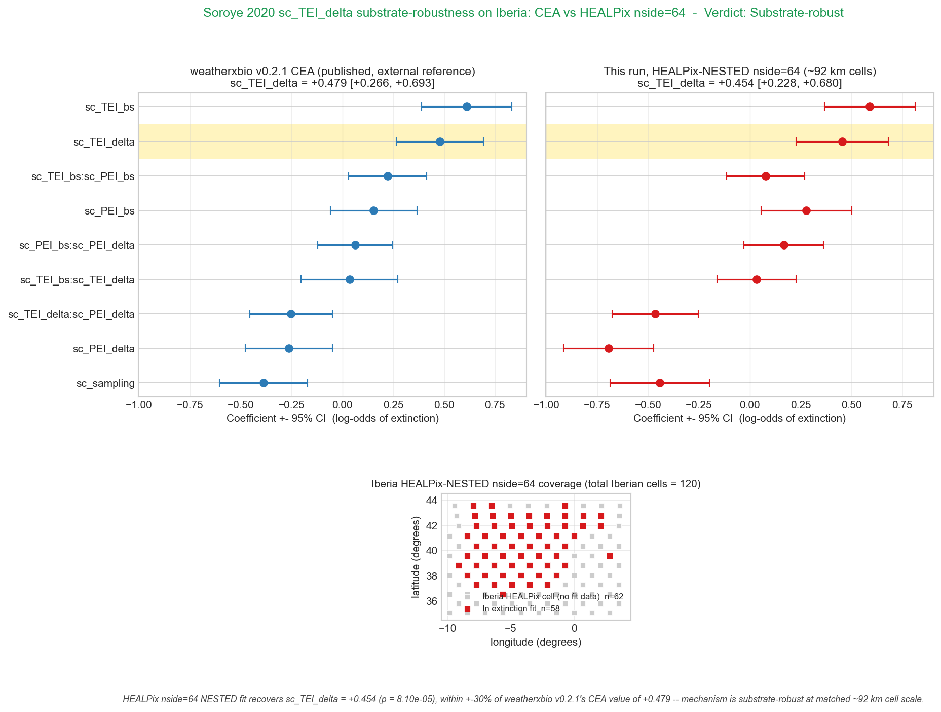
This chapter generates figures/main_result.png — a forest plot of the CEA-only Tier-1 GLMM coefficients for Iberian Bombus, intended as a Pass-1 sanity check that the Soroye et al. (2020) GLMM replicates on Iberian data with Soroye’s own CRU TS climate inputs.

The CEA-only PNG is intentionally not committed to the repo (see .gitignore). The canonical Tier-1 deliverable is the substrate-comparison figure in chapter 04h_figures_healpix, which shows the same coefficients side-by-side at CEA and HEALPix nside=64 and reports the substrate-robustness verdict. Reproducing the CEA-only figure here:

snakemake --cores 1 figures/main_result.png

Or by running this notebook directly:

jupyter execute --inplace notebooks/04_figures.ipynb

The headline Tier-1 visual (CEA + HEALPix side-by-side) is on the next chapter:

Tier-1 GLMM coefficient comparison: CEA vs HEALPix nside=64 — sc_TEI_delta is positive, large, and credible at both substrates (within 30%)