08 — Tier-2 projection figures (HEALPix nside=128, Option C) - weatherxbiodiversity-projection-nside128

Produces:

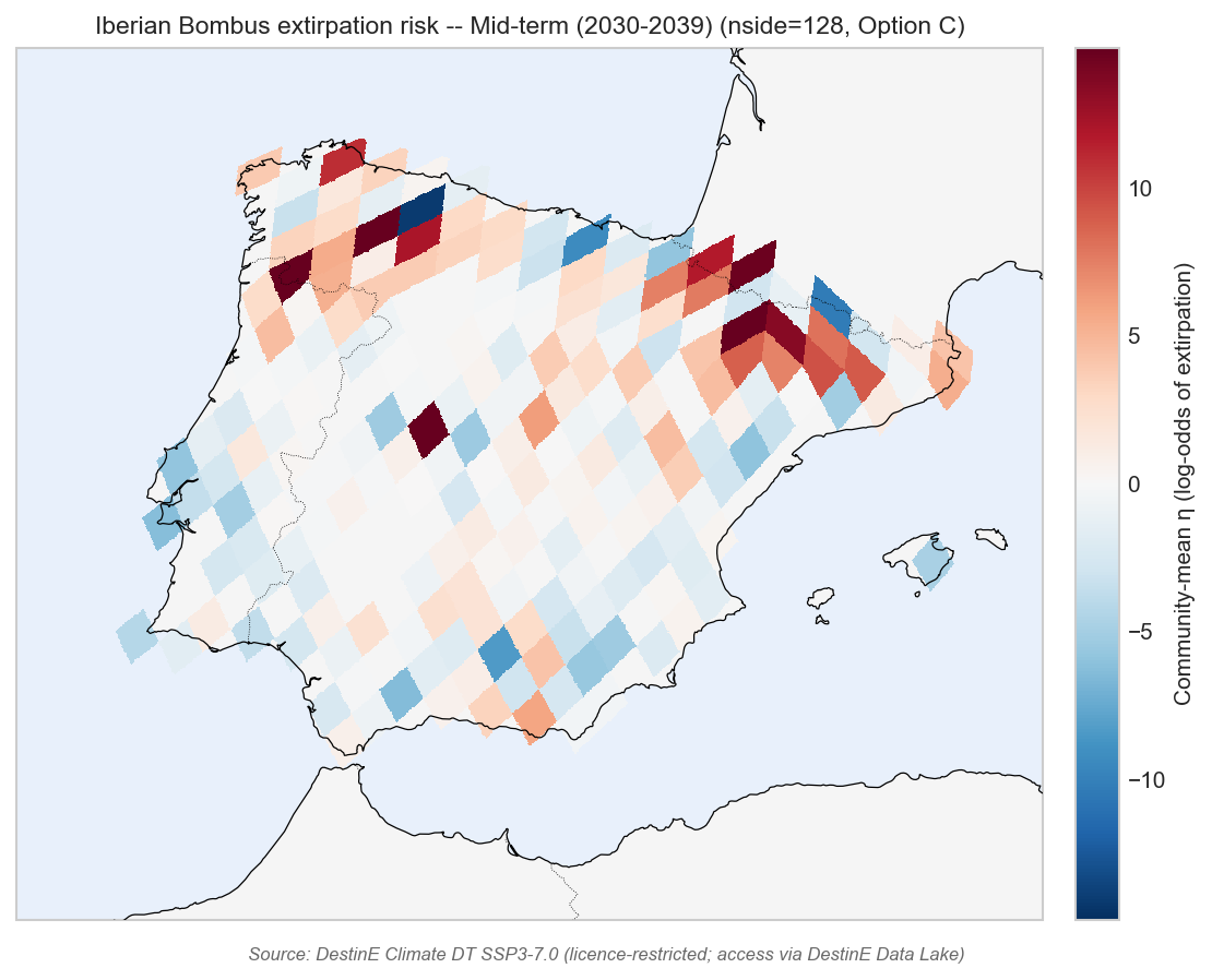
figures/projection_species_rank.png — two-panel ranked bar chart (near-term left, mid-term right) of per-species posterior-mean η (GLMM linear predictor / log-odds of extirpation) with 95 % HDI error bars; top-3 species per horizon highlighted in gold. η is reported instead of p = expit(η) because future predictors under SSP3-7.0 may still lie outside the Tier-1 training distribution where logit saturation makes p uninterpretable.
figures/projection_risk_map_2020_2029.png — Iberia HEALPix nside=128 risk map of community-mean η, RdBu_r diverging colormap centred on η = 0 (= moderate-risk threshold p = 0.5).
figures/projection_risk_map_2030_2039.png — same, mid-term.
figures/projection_proj_comparison_<horizon>.png — Mollweide-vs-LAEA side-by-side native-polygon comparison (methodological transparency).
figures/projection_summary.png — combined panel for the Jupyter Book / nanopub Outcome draft (rank chart + the more impactful map).

Per DOMAIN.md: HEALPix is always NESTED, and we use healpix-geo (NOT healpy) for the cell→lat/lon mapping, and healpix-plot for the canonical resampling-onto-cartopy bridge.

import json
from pathlib import Path

import cartopy.crs as ccrs
import cartopy.feature as cfeature
import matplotlib.pyplot as plt
import numpy as np
import xarray as xr
import healpix_plot
from healpix_plot import HealpixGrid
# healpix_geo.nested.vertices is the canonical way to get the 4 corners
# of each HEALPix cell on a chosen ellipsoid (sphere | WGS84). Used for
# the native-polygon rendering in the projection-comparison figure.
from healpix_geo.nested import vertices as hp_vertices
from matplotlib.collections import PolyCollection

plt.style.use("seaborn-v0_8-whitegrid")

ROOT = Path("..").resolve()
HPORT = ROOT / "healpix_port"
OUT_DIR = HPORT / "outputs_iberia"
RESULTS_DIR = ROOT / "results"
PRECOMP = ROOT / "data" / "precomputed"
FIG_DIR = ROOT / "figures"
FIG_DIR.mkdir(parents=True, exist_ok=True)

# Iberia nside=128 cells (depth=7, NESTED).
DEPTH = 7
IBERIA_PIX_128 = np.load(PRECOMP / "iberia_pix_nside128_nested.npy").astype(np.uint64)
N_128 = len(IBERIA_PIX_128)
print(f"Iberia HEALPix nside=128 cells: {N_128}")

Load projection summary + per-cell rasters¶

with open(RESULTS_DIR / "projection_headline.json") as f:
    summary = json.load(f)

HORIZONS = ["2020_2029", "2030_2039"]
HORIZON_TITLES = {
    "2020_2029": "Near-term (2020-2029)",
    "2030_2039": "Mid-term (2030-2039)",
}

per_cell = {}
for h in HORIZONS:
    p = RESULTS_DIR / f"projection_{h}.nc"
    if p.exists():
        ds_p = xr.open_dataset(p)
        per_cell[h] = ds_p["community_mean_eta"].values.astype(float)
        print(f"  loaded {p.name}: shape {per_cell[h].shape}")
    else:
        print(f"  [missing] {p}")

HEALPix plotting via `healpix_plot` (EOPF-DGGS canonical)¶

We use healpix_plot.plot() — the EOPF-DGGS-canonical HEALPix + cartopy plotting bridge (per DOMAIN.md: *"replaces ad-hoc ang2pix

pcolormesh bridges"*). Internally it:

Resamples the sparse nside=128 NESTED cells onto a dense regular lon/lat grid (nearest-neighbour by default) at the requested view extent.
Renders the resampled raster cleanly in any cartopy projection.

HPX_GRID = HealpixGrid(level=DEPTH, indexing_scheme="nested", ellipsoid="WGS84")
print(f"HealpixGrid: level={DEPTH} (nside={2**DEPTH}), NESTED, WGS84")

# Pre-compute the on-WGS84 cell vertices once. Used by the native-polygon
# rendering in the projection-comparison figure (lets cartopy reproject
# the WGS84 vertices through any target CRS).
_lon_v, _lat_v = hp_vertices(IBERIA_PIX_128, DEPTH, ellipsoid="WGS84")
_lon_v = np.where(_lon_v > 180.0, _lon_v - 360.0, _lon_v)
WGS84_POLY_XY = np.stack([_lon_v, _lat_v], axis=-1)   # (N_128, 4, 2)
print(f"WGS84 cell-vertex polygon array: shape={WGS84_POLY_XY.shape}")

Helper: ranked bar chart on a given matplotlib axis¶

GOLD = "#d4a017"
DARK_GOLD = "#8a6a0c"
TEAL = "#2c7bb6"
ORANGE = "#d7191c"
DATA_FOOTER = (
    "Source: DestinE Climate DT SSP3-7.0 "
    "(licence-restricted; access via DestinE Data Lake)"
)


def _plot_rank(ax, records, title, color, order_species=None,
               highlight_species=None):
    """Horizontal bar chart of per-species posterior-mean η (linear
    predictor / log-odds of extirpation under SSP3-7.0)."""
    by_name = {r["species"]: r for r in records}
    if order_species is not None:
        species = [sp for sp in order_species if sp in by_name]
    else:
        species = [r["species"] for r in records]

    means = np.array([by_name[sp]["post_mean_eta"] for sp in species])
    los = np.array([by_name[sp]["eta_hdi95_low"] for sp in species])
    his = np.array([by_name[sp]["eta_hdi95_high"] for sp in species])

    y = np.arange(len(species))
    err = np.vstack([means - los, his - means])

    if highlight_species is None:
        top3 = set(sorted(species, key=lambda s: -by_name[s]["post_mean_eta"])[:3])
    else:
        top3 = set(highlight_species)
    bar_colors = [DARK_GOLD if sp in top3 else color for sp in species]

    ax.barh(y, means, color=bar_colors, alpha=0.85, edgecolor="white")
    ax.errorbar(means, y, xerr=err, fmt="none", ecolor="black",
                elinewidth=0.8, capsize=2, alpha=0.5)
    ax.axvline(0, color="black", linewidth=0.6, linestyle="--", alpha=0.4)
    ax.set_yticks(y)
    ax.set_yticklabels([f"B. {sp}" for sp in species], fontsize=8)
    ax.invert_yaxis()
    ax.set_xlabel("Posterior-mean η (log-odds of extirpation)\n(95% HDI; η > 0 ↔ p > 0.5)")
    ax.set_title(title, fontsize=11)
    span = max(abs(means.min()), abs(means.max()))
    ax.set_xlim(-span * 1.15, span * 1.15)
    ax.grid(axis="x", linewidth=0.3, alpha=0.5)

Helper: HEALPix-cell map on a given cartopy axis¶

def _draw_healpix_map(ax, raster_per_cell, title):
    """Draw the Iberia raster via `healpix_plot.plot` (EOPF-DGGS canonical),
    in **ETRS89 / LAEA Europe (EPSG:3035)** — the canonical European
    biodiversity reporting CRS."""
    pc = ccrs.PlateCarree()
    ax.set_extent([-10.5, 4.5, 35.0, 44.5], crs=pc)
    ax.add_feature(cfeature.LAND, facecolor="#f5f5f5", zorder=0)
    ax.add_feature(cfeature.OCEAN, facecolor="#e8f0fb", zorder=0)

    valid = np.isfinite(raster_per_cell)
    if valid.sum() == 0:
        ax.set_title(title + " (no data)", fontsize=11)
        return None

    span = max(0.5, float(np.nanpercentile(np.abs(raster_per_cell), 98)))

    # `healpix_plot.plot` resamples the sparse NESTED cells onto a
    # regular grid at the requested `view` extent. shape=800 is ample
    # for a 14°×9° view at nside=128 (~46 km cells).
    img = healpix_plot.plot(
        cell_ids=IBERIA_PIX_128,
        data=raster_per_cell.astype(np.float64),
        healpix_grid=HPX_GRID,
        sampling_grid={"shape": 800},
        view=(-10.5, 4.5, 35.0, 44.5),
        interpolation="nearest",
        background_value=np.nan,
        ax=ax,
        cmap="RdBu_r",
        vmin=-span,
        vmax=+span,
        title=None,
    )
    ax.add_feature(cfeature.COASTLINE, linewidth=0.6, zorder=3)
    ax.add_feature(cfeature.BORDERS, linewidth=0.4, linestyle=":", zorder=3)
    ax.set_title(title, fontsize=11)
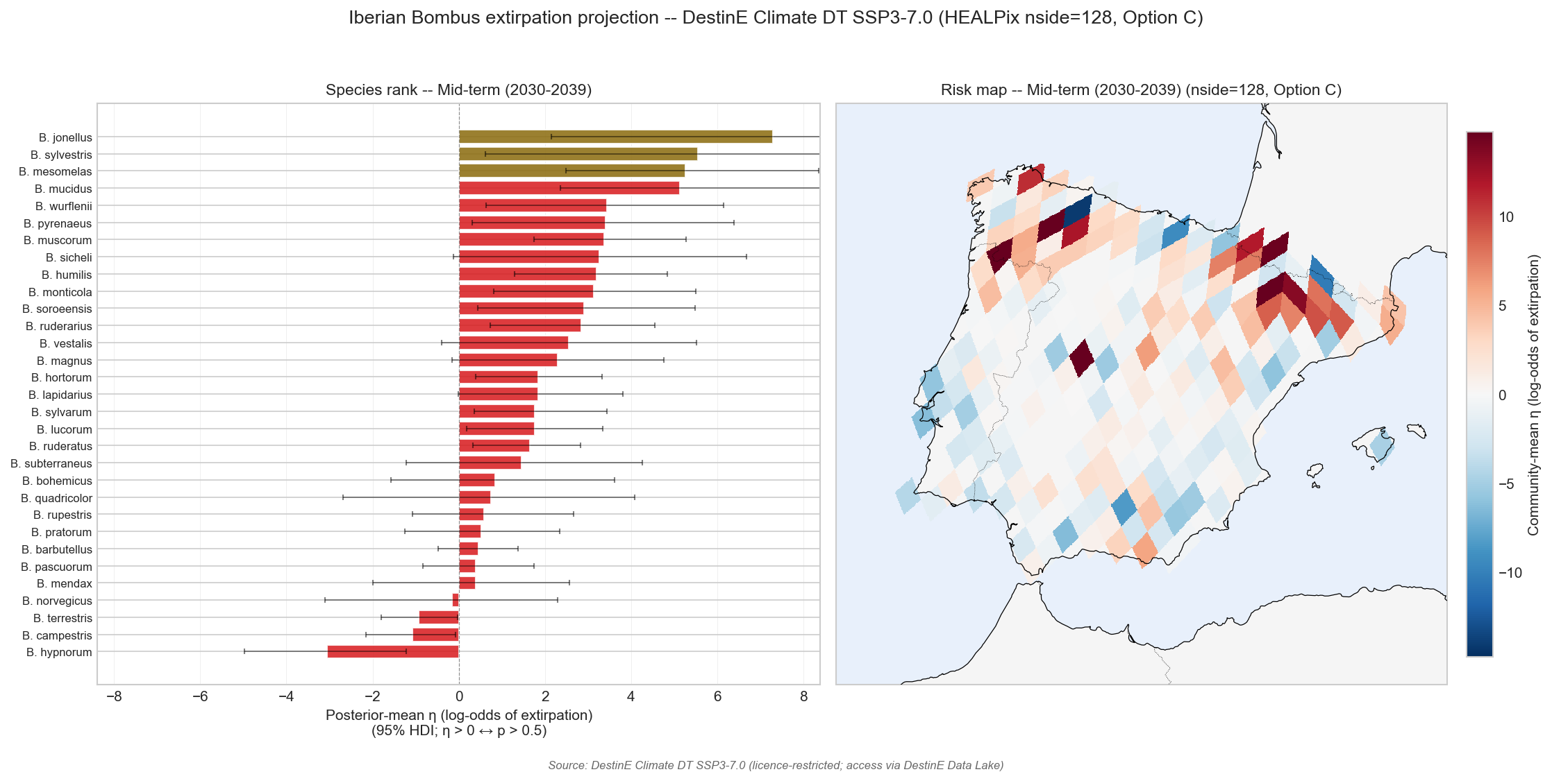
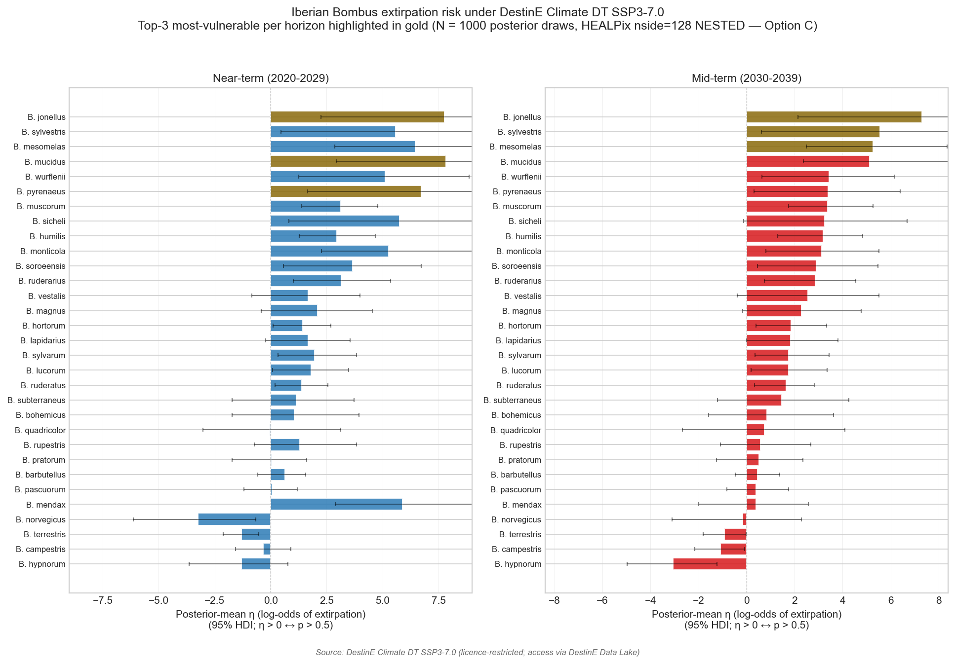
    return img

Figure 1 — species-rank chart (two panels)¶

fig, axes = plt.subplots(1, 2, figsize=(13, 9), sharey=False)
records_near = summary["horizons"]["2020_2029"]["species_ranked"]
records_mid = summary["horizons"]["2030_2039"]["species_ranked"]


def _top3_species(records):
    return [r["species"] for r in
            sorted(records, key=lambda r: -r["post_mean_eta"])[:3]]


mid_order = [
    r["species"] for r in
    sorted(records_mid, key=lambda r: -r["post_mean_eta"])
]
top3_near = set(_top3_species(records_near))
top3_mid = set(_top3_species(records_mid))

_plot_rank(axes[0], records_near, HORIZON_TITLES["2020_2029"], TEAL,
           order_species=mid_order, highlight_species=top3_near)
_plot_rank(axes[1], records_mid, HORIZON_TITLES["2030_2039"], ORANGE,
           order_species=mid_order, highlight_species=top3_mid)
fig.suptitle(
    "Iberian Bombus extirpation risk under DestinE Climate DT SSP3-7.0\n"
    f"Top-3 most-vulnerable per horizon highlighted in gold "
    f"(N = {summary['method']['n_posterior_draws']} posterior draws, "
    f"HEALPix nside=128 NESTED — Option C)",
    fontsize=12,
)
fig.text(
    0.5, 0.005, DATA_FOOTER,
    ha="center", va="bottom", fontsize=8, color="dimgray", style="italic",
)
fig.tight_layout(rect=[0, 0.03, 1, 0.95])
out = FIG_DIR / "projection_species_rank.png"
fig.savefig(out, dpi=150, bbox_inches="tight")
plt.show()
print(f"Saved {out}")

Native-polygon HEALPix-on-WGS84 helper¶

Renders the nside=128 cells as their actual on-WGS84 quadrilateral polygons (vertices from healpix_geo.nested.vertices(..., ellipsoid="WGS84")). Lets cartopy reproject the polygon edges into whatever the axis CRS is.

def _draw_healpix_polygons_native(ax, raster_per_cell, title):
    """Render HEALPix cells as their native WGS84-ellipsoid polygons,
    reprojected by cartopy into the axis's CRS."""
    pc = ccrs.PlateCarree()
    ax.set_extent([-10.5, 4.5, 35.0, 44.5], crs=pc)
    ax.add_feature(cfeature.LAND, facecolor="#f5f5f5", zorder=0)
    ax.add_feature(cfeature.OCEAN, facecolor="#e8f0fb", zorder=0)

    valid = np.isfinite(raster_per_cell)
    if valid.sum() == 0:
        ax.set_title(title + " (no data)", fontsize=11)
        return None

    span = max(0.5, float(np.nanpercentile(np.abs(raster_per_cell), 98)))

    polys = WGS84_POLY_XY[valid]
    vals = raster_per_cell[valid]
    pcoll = PolyCollection(
        polys,
        array=vals,
        cmap="RdBu_r",
        norm=plt.Normalize(vmin=-span, vmax=+span),
        edgecolors="black",
        linewidths=0.15,
        transform=pc,           # vertices are WGS84 lon/lat → reproject via PlateCarree CRS
        zorder=1,
    )
    ax.add_collection(pcoll)
    ax.add_feature(cfeature.COASTLINE, linewidth=0.6, zorder=3)
    ax.add_feature(cfeature.BORDERS, linewidth=0.4, linestyle=":", zorder=3)
    ax.set_title(title, fontsize=11)
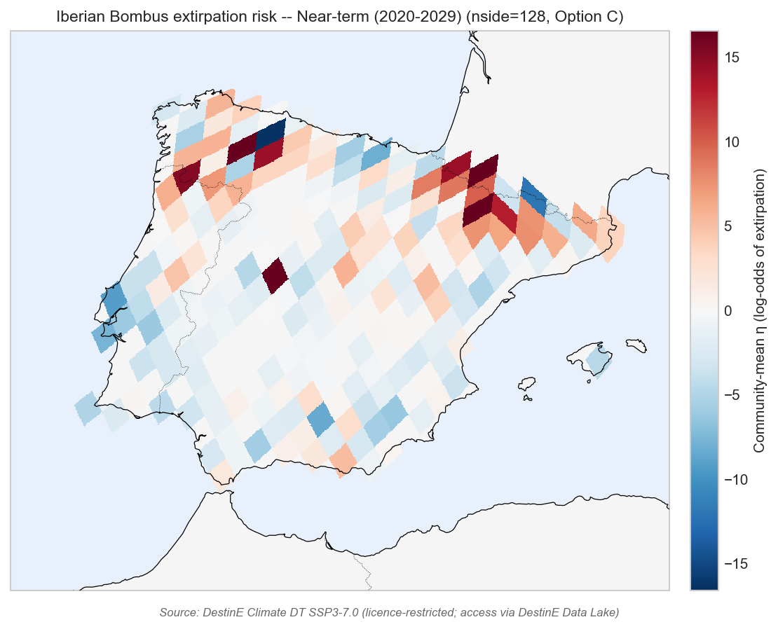
    return pcoll

Figures 2 + 3 — per-cell community-mean risk maps (LAEA Europe)¶


def _plot_map(horizon: str, raster: np.ndarray) -> Path:
    proj = ccrs.epsg(3035)
    fig = plt.figure(figsize=(7.5, 6))
    ax = plt.axes(projection=proj)
    pc = _draw_healpix_map(
        ax, raster,
        f"Iberian Bombus extirpation risk -- {HORIZON_TITLES[horizon]} "
        "(nside=128, Option C)",
    )
    if pc is not None:
        cbar = plt.colorbar(pc, ax=ax, orientation="vertical",
                            fraction=0.04, pad=0.03)
        cbar.set_label("Community-mean η (log-odds of extirpation)")
    fig.text(
        0.5, 0.01, DATA_FOOTER,
        ha="center", va="bottom", fontsize=8, color="dimgray", style="italic",
    )
    fig.tight_layout(rect=[0, 0.03, 1, 1])
    out = FIG_DIR / f"projection_risk_map_{horizon}.png"
    fig.savefig(out, dpi=150, bbox_inches="tight")
    plt.show()
    return out


for h in HORIZONS:
    if h not in per_cell:
        print(f"  [skip] {h}")
        continue
    out = _plot_map(h, per_cell[h])
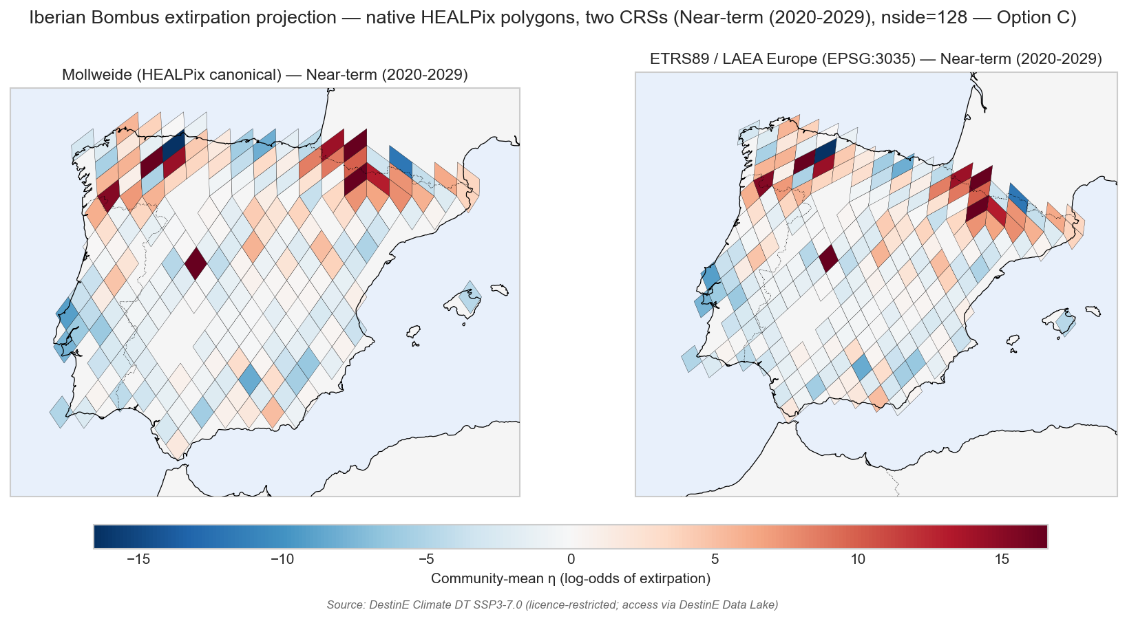
    print(f"Saved {out}")

Projection comparison — native HEALPix-on-WGS84 polygons in two CRSs¶

Same physical HEALPix cells, rendered as native polygons, reprojected by cartopy into Mollweide (HEALPix canonical) and ETRS89 / LAEA Europe (EPSG:3035). Methodological transparency: equal-area in both projections.

def _plot_proj_comparison(horizon: str, raster: np.ndarray) -> Path:
    fig = plt.figure(figsize=(14, 6))
    ax_left = fig.add_subplot(1, 2, 1, projection=ccrs.Mollweide())
    ax_right = fig.add_subplot(1, 2, 2, projection=ccrs.epsg(3035))

    pc_left = _draw_healpix_polygons_native(
        ax_left, raster,
        f"Mollweide (HEALPix canonical) — {HORIZON_TITLES[horizon]}",
    )
    pc_right = _draw_healpix_polygons_native(
        ax_right, raster,
        f"ETRS89 / LAEA Europe (EPSG:3035) — {HORIZON_TITLES[horizon]}",
    )

    if pc_right is not None:
        cbar = fig.colorbar(
            pc_right, ax=[ax_left, ax_right], orientation="horizontal",
            fraction=0.05, pad=0.06, aspect=40,
        )
        cbar.set_label("Community-mean η (log-odds of extirpation)")

    fig.suptitle(
        f"Iberian Bombus extirpation projection — native HEALPix polygons, "
        f"two CRSs ({HORIZON_TITLES[horizon]}, nside=128 — Option C)",
        fontsize=13,
    )
    fig.text(
        0.5, 0.01, DATA_FOOTER,
        ha="center", va="bottom", fontsize=8, color="dimgray", style="italic",
    )
    out = FIG_DIR / f"projection_proj_comparison_{horizon}.png"
    fig.savefig(out, dpi=150, bbox_inches="tight")
    plt.show()
    return out


for h in HORIZONS:
    if h not in per_cell:
        continue
    out = _plot_proj_comparison(h, per_cell[h])
    print(f"Saved {out}")

Figure 4 — combined summary panel for the Jupyter Book¶

def _median_risk(h):
    if h not in per_cell:
        return -np.inf
    arr = per_cell[h]
    finite = arr[np.isfinite(arr)]
    return float(np.median(finite)) if finite.size else -np.inf


impactful = "2030_2039"
if per_cell:
    impactful = max(per_cell.keys(), key=_median_risk)
print(f"Combined panel uses {impactful} for the map "
      f"(median community risk = {_median_risk(impactful):.3f}).")

fig = plt.figure(figsize=(15, 7.5))
gs = fig.add_gridspec(1, 2, width_ratios=[1.1, 1.0])

ax_rank = fig.add_subplot(gs[0, 0])
records = summary["horizons"][impactful]["species_ranked"]
_plot_rank(
    ax_rank, records,
    f"Species rank -- {HORIZON_TITLES[impactful]}",
    ORANGE if impactful == "2030_2039" else TEAL,
)

if impactful in per_cell:
    ax_map = fig.add_subplot(gs[0, 1], projection=ccrs.epsg(3035))
    pc = _draw_healpix_map(
        ax_map, per_cell[impactful],
        f"Risk map -- {HORIZON_TITLES[impactful]} (nside=128, Option C)",
    )
    if pc is not None:
        plt.colorbar(
            pc, ax=ax_map, orientation="vertical",
            fraction=0.04, pad=0.03,
            label="Community-mean η (log-odds of extirpation)",
        )

fig.suptitle(
    "Iberian Bombus extirpation projection -- DestinE Climate DT SSP3-7.0 "
    "(HEALPix nside=128, Option C)",
    fontsize=13,
)
fig.text(
    0.5, 0.005, DATA_FOOTER,
    ha="center", va="bottom", fontsize=8, color="dimgray", style="italic",
)
fig.tight_layout(rect=[0, 0.03, 1, 0.95])
out = FIG_DIR / "projection_summary.png"
fig.savefig(out, dpi=150, bbox_inches="tight")
plt.show()
print(f"Saved {out}")

Tier-2 figures (committed; CI-renderable)¶

Tier-2 notebooks 05–08 require DestinE Climate DT credentials, so this chapter cannot execute on a generic GitHub Actions runner. The figures below are the committed PNGs from the local DestinE-platform run.