This worked example shows the GRID4EARTH analysis stack end to end:
read a real Sentinel-2 L2A surface-reflectance scene (a Cloud-Optimized GeoTIFF on AWS, no credentials needed);
put it on an equal-area HEALPix grid on the WGS84 ellipsoid with
healpix-geo;compute its isotropic power spectrum with
healpix-analyse— a differentiable (PyTorch) toolkit for analysing signals on HEALPix grids.
The power spectrum tells us at which spatial scales the scene has structure —
the size of fields, texture, edges. Doing it on an equal-area grid matters: a
naïve lon/lat grid shrinks cells towards the poles, which biases the spectrum;
HEALPix cells all cover the same surface area (depth N → nside = 2**N), so
the spectrum is unbiased.
import json
import os
import numpy as np
import matplotlib.pyplot as plt
import rasterio
from rasterio.windows import Window
from pyproj import Transformer
from scipy.ndimage import map_coordinates
from scipy.signal.windows import tukey

import healpix_geo
from healpix_analyse.make_rectangle import make_healpix_rectangle_from_lonlat
from healpix_analyse.resample import resample_to_latlon_grid
from healpix_analyse.ps import ps
1. Read a Sentinel-2 L2A scene
Scene S2A_22WEV_20190723 (tile T22WEV, 2019-07-23) over south-west Greenland,
from the public Element 84 / AWS sentinel-s2-l2a-cogs archive. We read a small
window of the 10 m red band (B04) straight from the COG — only the bytes we need.
BASE = (
    "https://sentinel-cogs.s3.us-west-2.amazonaws.com/sentinel-s2-l2a-cogs/"
    "22/W/EV/2019/7/S2A_22WEV_20190723_0_L2A"
)
COL_OFF, ROW_OFF, SIZE = 9900, 7050, 256  # 256 px @ 10 m ≈ 2.6 km square

with rasterio.open(f"{BASE}/B04.tif") as src:
    window = Window(COL_OFF, ROW_OFF, SIZE, SIZE)
    s2 = src.read(1, window=window).astype(float)
    transform = src.window_transform(window)  # UTM affine for this window
    crs = src.crs                             # EPSG:32622 (UTM zone 22N)

print(f"Sentinel-2 B04 window: {s2.shape}, CRS {crs}")
Sentinel-2 B04 window: (256, 256), CRS EPSG:32622
/tmp/ipykernel_2417/1527305605.py:9: DeprecationWarning: Setting the shape on a NumPy array has been deprecated in NumPy 2.5.
As an alternative, you can create a new view using np.reshape (with copy=False if needed).
  s2 = src.read(1, window=window).astype(float)
fig, ax = plt.subplots(figsize=(5, 5))
im = ax.imshow(s2, cmap="magma")
ax.set_title("Sentinel-2 B04 (red) reflectance — raw UTM window")
ax.set_axis_off()
fig.colorbar(im, ax=ax, shrink=0.8, label="reflectance (DN)")
plt.show()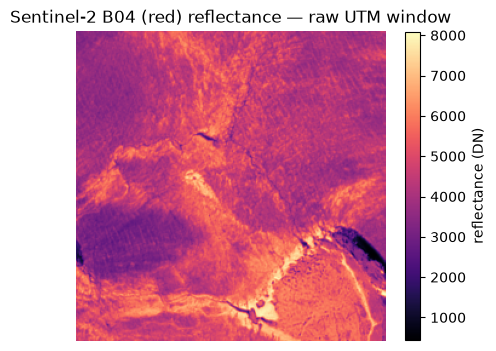
2. Put the scene on an equal-area HEALPix grid (healpix-geo, WGS84)
We build the HEALPix cells that tile this window’s lon/lat bounding box at
depth = 18 (~25 m cells), then sample the Sentinel-2 reflectance at each cell
centre. healpix-geo evaluates the cell geometry on the WGS84 ellipsoid.
DEPTH = 18
ELLIPSOID = "WGS84"

# window lon/lat bounding box (UTM corners -> WGS84)
to_lonlat = Transformer.from_crs(crs, "EPSG:4326", always_xy=True)
xs = [transform.c, transform.c + SIZE * transform.a]
ys = [transform.f + SIZE * transform.e, transform.f]
corners = [to_lonlat.transform(x, y) for x in xs for y in ys]
lons, lats = zip(*corners)
bbox = (min(lons), min(lats), max(lons), max(lats))

# HEALPix cells covering the bbox, as a 2-D rectangle of cell ids
cell_ids_2d = make_healpix_rectangle_from_lonlat(bbox=bbox, level=DEPTH, ellipsoid=ELLIPSOID)
cell_lon, cell_lat = healpix_geo.ring.healpix_to_lonlat(
    cell_ids_2d.flatten(), DEPTH, ellipsoid=ELLIPSOID
)

# sample S2 at each cell centre: WGS84 -> UTM -> array index -> bilinear value
to_utm = Transformer.from_crs("EPSG:4326", crs, always_xy=True)
cell_x, cell_y = to_utm.transform(cell_lon, cell_lat)
col = (cell_x - transform.c) / transform.a
row = (cell_y - transform.f) / transform.e
field = map_coordinates(s2, [row, col], order=1, mode="nearest").reshape(cell_ids_2d.shape)

print(f"HEALPix rectangle at depth {DEPTH} (nside={2**DEPTH}): {cell_ids_2d.shape} cells")
HEALPix rectangle at depth 18 (nside=262144): (133, 88) cells
fig, ax = plt.subplots(figsize=(5.5, 4.5))
sc = ax.scatter(cell_lon, cell_lat, c=field.flatten(), s=4, cmap="magma")
ax.set_xlabel("Longitude")
ax.set_ylabel("Latitude")
ax.set_title(f"Sentinel-2 B04 on equal-area HEALPix cells (depth {DEPTH}, WGS84)")
fig.colorbar(sc, ax=ax, label="reflectance (DN)")
plt.show()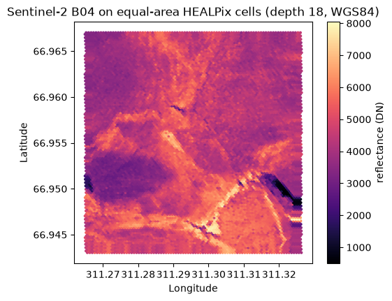
3. Isotropic power spectrum (healpix-analyse)
We resample the HEALPix field back to a regular grid, apodise it with a Tukey
window (to suppress edge leakage), and compute the radially-averaged 2-D power
spectrum with healpix-analyse’s ps. The result is power vs spatial
frequency — the scene’s structure as a function of scale.
lat_2d = cell_lat.reshape(cell_ids_2d.shape)
lon_2d = cell_lon.reshape(cell_ids_2d.shape)
gridded = np.nan_to_num(resample_to_latlon_grid(lat_2d, lon_2d, field, method="cubic"))

alpha = 0.2
apod = tukey(gridded.shape[0], alpha)[:, None] * tukey(gridded.shape[1], alpha)[None, :]
freqs, spectrum = ps(apod * (gridded - gridded.mean()))
freqs, spectrum = np.asarray(freqs), np.asarray(spectrum)
fig, ax = plt.subplots(figsize=(6, 4))
ax.loglog(freqs[1:], spectrum[1:], "o-", color="#0072B2")
ax.set_xlabel("spatial frequency (cycles / cell)")
ax.set_ylabel("power")
ax.set_title("Isotropic power spectrum of the Sentinel-2 scene on HEALPix")
ax.grid(True, which="both", alpha=0.3)
fig.tight_layout()
# Persist the figure as a research-object output (Snakemake target).
os.makedirs("results", exist_ok=True)
fig.savefig("results/powerspectrum.png", dpi=150, bbox_inches="tight")
plt.show()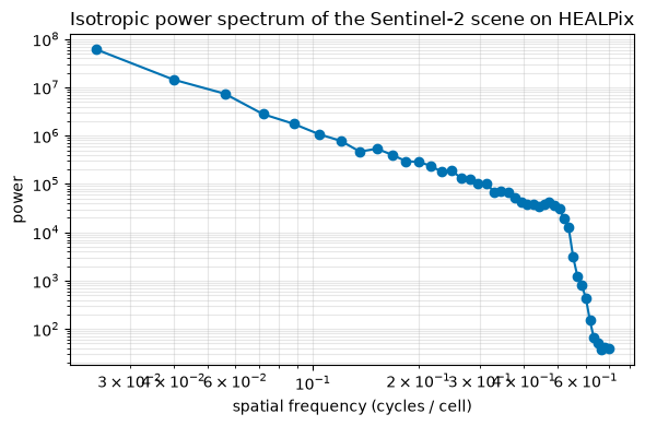
What this shows
The spectrum falls off with frequency — most of the scene’s variance is at large
spatial scales, with progressively less power at finer scales, the hallmark of a
natural surface-reflectance field. Because every HEALPix cell covers the same
area on the WGS84 ellipsoid, this spectrum is free of the latitude-dependent
area bias a lon/lat grid would introduce — which is exactly what the GRID4EARTH
stack (healpix-geo for the grid, healpix-analyse for the analysis) is for.
Because healpix-analyse is built on PyTorch, every operator here is
differentiable, so this same pipeline drops straight into a learning loop.
# Headline numbers, for the record. Written to results/ as a research-object
# output so the Snakemake workflow has a concrete, citable target.
summary = {
    "scene": "S2A_22WEV_20190723",
    "band": "B04 (red, 10 m)",
    "window_px": [COL_OFF, ROW_OFF, SIZE],
    "healpix_depth": DEPTH,
    "healpix_nside": 2**DEPTH,
    "ellipsoid": ELLIPSOID,
    "healpix_cells": int(cell_ids_2d.size),
    "spectrum_points": int(spectrum.size),
}
os.makedirs("results", exist_ok=True)
with open("results/powerspectrum.json", "w") as fh:
    json.dump(summary, fh, indent=2)
print(json.dumps(summary, indent=2))
{
"scene": "S2A_22WEV_20190723",
"band": "B04 (red, 10 m)",
"window_px": [
9900,
7050,
256
],
"healpix_depth": 18,
"healpix_nside": 262144,
"ellipsoid": "WGS84",
"healpix_cells": 11704,
"spectrum_points": 44
}