What this notebook does
This notebook reproduces the core result of Delouis et al. (2022, A&A): the Cross Scattering Transform captures non-Gaussian statistics of astrophysical images and can synthesize new realizations that share those statistics.
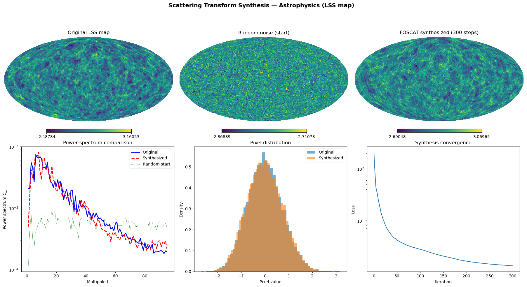
We use a Large Scale Structure (LSS) cosmological map on a HEALPix sphere and show that FOSCAT can generate a new map from random noise that has the same multi-scale statistical properties as the original.
The claim we reproduce
“Non-Gaussian modelling and statistical denoising of Planck dust polarization full-sky maps using scattering transforms” — Delouis et al. 2022, A&A 668, A122
The paper demonstrates that scattering transforms capture higher-order (non-Gaussian) statistics of astrophysical images on the sphere — going beyond the power spectrum which only captures second-order (Gaussian) statistics. This enables both denoising and synthesis of realistic astrophysical maps.
Credits
Method and FOSCAT software: Jean-Marc Delouis, LOPS/CNRS
Demo data (LSS map): FOSCAT_DEMO repository
This reproduction: Anne Fouilloux, LifeWatch ERIC (FIESTA-OSCARS)
import os
os.environ["KMP_DUPLICATE_LIB_OK"] = "TRUE"

import numpy as np
import healpy as hp
import foscat.scat_cov as sc
import foscat.Synthesis as synthe
import matplotlib.pyplot as plt
from pathlib import Path
import json
import time
Configuration
RESULTS = Path("results")
RESULTS.mkdir(exist_ok=True)

# HEALPix resolution — higher = more pixels, slower
# nside=8 (768 px): ~2s, quick test
# nside=32 (12k px): ~5min
# nside=64 (49k px): ~30min on CPU
# nside=128 (196k px): needs GPU
CI_MODE = os.environ.get("CI", "").lower() in ("true", "1")
NSIDE = 8 if CI_MODE else 32
NSTEPS = 50 if CI_MODE else 300
SEED = 1234
1. Load astrophysics data
The Large Scale Structure (LSS) map represents the cosmic density field — the distribution of matter in the universe. It has complex non-Gaussian structure (filaments, voids, clusters) that cannot be fully described by the power spectrum alone.
import urllib.request

data_path = Path("data/LSS_map_nside128.npy")

if not data_path.exists():
    print("Downloading LSS map from FOSCAT_DEMO...")
    data_path.parent.mkdir(parents=True, exist_ok=True)
    url = "https://github.com/jmdelouis/FOSCAT_DEMO/raw/main/data/LSS_map_nside128.npy"
    urllib.request.urlretrieve(url, str(data_path))
    print(f"  Downloaded: {data_path.stat().st_size / 1e6:.1f} MB")

print("Loading LSS map...")
im_full = np.load(str(data_path))
print(f"  Original: nside=128, npix={im_full.shape[0]:,}")

# Downgrade to working resolution
im = hp.ud_grade(im_full, NSIDE, order_in='NESTED', order_out='NESTED')
im = im.reshape(1, 12 * NSIDE**2).astype(np.float32)
print(f"  Working: nside={NSIDE}, npix={im.shape[1]:,}")
print(f"  Data range: {im.min():.4f} to {im.max():.4f}")
print(f"  Mean: {im.mean():.4f}, Std: {im.std():.4f}")
Loading LSS map...
Original: nside=128, npix=196,608
Working: nside=32, npix=12,288
Data range: -2.4878 to 3.1605
Mean: -0.0000, Std: 0.7392
2. Create random starting point
FOSCAT starts from random noise and iteratively adjusts it until its scattering transform coefficients match those of the target map. The result is a new map that is visually different from the original but shares the same statistical properties.
np.random.seed(SEED)
imap = np.random.randn(*im.shape).astype(np.float32)
imap = imap * im.std() + im.mean()

print(f"Random start: mean={imap.mean():.4f}, std={imap.std():.4f}")

# No mask — use all pixels
mask = np.ones_like(im)
Random start: mean=0.0112, std=0.7370
3. Compute reference scattering coefficients
The scattering transform computes multi-scale wavelet coefficients and their correlations. These capture the texture, filamentary structure, and non-Gaussian statistics of the map.
We compute these from the original LSS map — this is what the synthesis will try to match.
print("Computing scattering coefficients...")
scat_op = sc.funct(NORIENT=4, KERNELSZ=3, all_type='float32', silent=True)
print(f"  Device: {scat_op.backend.device}")

ref, sref = scat_op.eval(im, mask=mask, calc_var=True)
print("  Reference scattering coefficients computed")
Computing scattering coefficients...
Device: cpu
/home/runner/micromamba/envs/fiesta-scattering-astro/lib/python3.11/site-packages/foscat/BkTorch.py:1329: UserWarning: The given NumPy array is not writable, and PyTorch does not support non-writable tensors. This means writing to this tensor will result in undefined behavior. You may want to copy the array to protect its data or make it writable before converting it to a tensor. This type of warning will be suppressed for the rest of this program. (Triggered internally at /home/conda/feedstock_root/build_artifacts/libtorch_1772252348570/work/torch/csrc/utils/tensor_numpy.cpp:213.)
  x = self.backend.from_numpy(x).to(self.torch_device)
/home/runner/micromamba/envs/fiesta-scattering-astro/lib/python3.11/site-packages/foscat/BkTorch.py:902: UserWarning: Sparse CSR tensor support is in beta state. If you miss a functionality in the sparse tensor support, please submit a feature request to https://github.com/pytorch/pytorch/issues. (Triggered internally at /home/conda/feedstock_root/build_artifacts/libtorch_1772252348570/work/aten/src/ATen/SparseCsrTensorImpl.cpp:49.)
  return self.backend.sparse_coo_tensor(indice, w, dense_shape).coalesce().to_sparse_csr().to(self.torch_device)
initialise down 32
initialise down 16
initialise down 8
initialise down 4
initialise down 2
  Reference scattering coefficients computed
4. Define loss function and synthesis
The loss measures how different the current map’s scattering coefficients are from the reference, normalized by the variance. FOSCAT minimizes this loss by adjusting pixel values.
def The_loss(x, scat_operator, args):
    ref = args[0]
    mask = args[1]
    sref = args[2]
    learn = scat_operator.eval(x, mask=mask)
    loss = scat_operator.reduce_mean(scat_operator.square((ref - learn) / sref))
    return loss

loss1 = synthe.Loss(The_loss, scat_op, ref, mask, sref)
sy = synthe.Synthesis([loss1])
5. Run synthesis
Starting from random noise, FOSCAT iteratively updates the map to match the scattering statistics of the original LSS map.
print(f"Running synthesis: {NSTEPS} steps, nside={NSIDE}...")
t0 = time.time()

omap = sy.run(
    scat_op.backend.bk_cast(imap),
    EVAL_FREQUENCY=max(NSTEPS // 10, 1),
    NUM_EPOCHS=NSTEPS,
    do_lbfgs=True
)

elapsed = time.time() - t0
omap_np = np.array(omap) if not hasattr(omap, 'numpy') else omap.numpy()
print(f"  Completed in {elapsed:.1f}s")
Running synthesis: 300 steps, nside=32...
Total number of loss 1
Itt 0 L= 208 ( 208 ) 0.221s
Itt 30 L= 6.6 ( 6.6 ) 7.475s
Itt 60 L= 3.71 ( 3.71 ) 6.827s
Itt 90 L= 2.94 ( 2.94 ) 7.538s
Itt 120 L= 2.44 ( 2.44 ) 6.851s
Itt 150 L= 2.06 ( 2.06 ) 6.613s
Itt 180 L= 1.78 ( 1.78 ) 7.054s
Itt 210 L= 1.59 ( 1.59 ) 6.839s
Itt 240 L= 1.47 ( 1.47 ) 6.588s
Itt 270 L= 1.39 ( 1.39 ) 6.593s
Itt 300 L= 1.33 ( 1.33 ) 6.574s
Final Loss  1.3332691192626953
  Completed in 69.2s
6. Validate results
We check that the synthesized map has the same statistical properties as the original, even though it looks visually different.
# Basic statistics
print("=== Validation ===")
print(f"  {'':20s} {'Original':>12s} {'Synthesized':>12s}")
print(f"  {'Mean':20s} {im.mean():12.4f} {omap_np.mean():12.4f}")
print(f"  {'Std':20s} {im.std():12.4f} {omap_np.std():12.4f}")
print(f"  {'Min':20s} {im.min():12.4f} {omap_np.min():12.4f}")
print(f"  {'Max':20s} {im.max():12.4f} {omap_np.max():12.4f}")

# Pixel-level correlation (should be LOW — not a copy)
corr = np.corrcoef(im.ravel(), omap_np.ravel())[0, 1]
print(f"  {'Pixel correlation':20s} {corr:12.4f}")
print(f"  (Low correlation expected — synthesized map is a NEW realization)")

# Power spectrum comparison
cl_orig = hp.anafast(hp.reorder(im[0], n2r=True))
cl_synth = hp.anafast(hp.reorder(omap_np[0], n2r=True))
cl_start = hp.anafast(hp.reorder(imap[0], n2r=True))

ps_ratio = np.mean(cl_synth[1:] / (cl_orig[1:] + 1e-20))
print(f"  {'Power spectrum ratio':20s} {ps_ratio:12.4f}")
print(f"  (Close to 1.0 = same large-scale structure)")

# Scattering coefficient comparison
out_scat = scat_op.eval(omap_np, mask=mask)
start_scat = scat_op.eval(imap, mask=mask)

ref_s1 = scat_op.backend.to_numpy(ref.S1)
out_s1 = scat_op.backend.to_numpy(out_scat.S1)
start_s1 = scat_op.backend.to_numpy(start_scat.S1)

scat_error_start = np.mean((ref_s1 - start_s1)**2)
scat_error_out = np.mean((ref_s1 - out_s1)**2)
improvement = (1 - scat_error_out / scat_error_start) * 100

print(f"  {'Scat coeff error (start)':20s} {scat_error_start:12.6f}")
print(f"  {'Scat coeff error (synth)':20s} {scat_error_out:12.6f}")
print(f"  {'Improvement':20s} {improvement:11.1f}%")
=== Validation ===
Original Synthesized
Mean -0.0000 0.0002
Std 0.7392 0.7447
Min -2.4878 -2.6905
Max 3.1605 3.0696
Pixel correlation -0.0120
(Low correlation expected — synthesized map is a NEW realization)
Power spectrum ratio 0.9833
(Close to 1.0 = same large-scale structure)
  Scat coeff error (start)     0.000857
  Scat coeff error (synth)     0.000003
  Improvement                 99.6%
7. Save results
results = {
    "method": "Cross Scattering Transform (FOSCAT)",
    "original_paper": "Delouis et al. 2022, A&A 668, A122",
    "original_paper_doi": "10.1051/0004-6361/202244566",
    "domain": "astrophysics",
    "data": "Large Scale Structure (LSS) cosmological map",
    "nside": NSIDE,
    "nsteps": NSTEPS,
    "elapsed_seconds": elapsed,
    "device": str(scat_op.backend.device),
    "statistics": {
        "original_mean": float(im.mean()),
        "original_std": float(im.std()),
        "synthesized_mean": float(omap_np.mean()),
        "synthesized_std": float(omap_np.std()),
        "pixel_correlation": float(corr),
        "power_spectrum_ratio": float(ps_ratio),
        "scattering_error_start": float(scat_error_start),
        "scattering_error_synth": float(scat_error_out),
        "scattering_improvement_pct": float(improvement),
    },
}

with open(RESULTS / "astro_synthesis_results.json", "w") as f:
    json.dump(results, f, indent=2)
print(f"Results saved: {RESULTS / 'astro_synthesis_results.json'}")
Results saved: results/astro_synthesis_results.json
# Plots
fig = plt.figure(figsize=(18, 10))

# Row 1: Maps
hp.mollview(im[0], nest=True, title='Original LSS map',
            sub=(2, 3, 1), fig=fig.number, cmap='viridis')
hp.mollview(imap[0], nest=True, title='Random noise (start)',
            sub=(2, 3, 2), fig=fig.number, cmap='viridis')
hp.mollview(omap_np[0], nest=True, title=f'FOSCAT synthesized ({NSTEPS} steps)',
            sub=(2, 3, 3), fig=fig.number, cmap='viridis')

# Row 2: Diagnostics
ax4 = fig.add_subplot(2, 3, 4)
ell = np.arange(len(cl_orig))
ax4.semilogy(ell[1:], cl_orig[1:], 'b-', label='Original', linewidth=2)
ax4.semilogy(ell[1:], cl_synth[1:], 'r--', label='Synthesized', linewidth=2)
ax4.semilogy(ell[1:], cl_start[1:], 'g:', label='Random start', linewidth=1)
ax4.set_xlabel('Multipole l')
ax4.set_ylabel('Power spectrum C_l')
ax4.set_title('Power spectrum comparison')
ax4.legend()

ax5 = fig.add_subplot(2, 3, 5)
bins = 50
ax5.hist(im.ravel(), bins=bins, alpha=0.6, label='Original', density=True)
ax5.hist(omap_np.ravel(), bins=bins, alpha=0.6, label='Synthesized', density=True)
ax5.set_xlabel('Pixel value')
ax5.set_ylabel('Density')
ax5.set_title('Pixel distribution')
ax5.legend()

ax6 = fig.add_subplot(2, 3, 6)
history = sy.get_history()
valid = history[history > 0]
ax6.semilogy(valid)
ax6.set_xlabel('Iteration')
ax6.set_ylabel('Loss')
ax6.set_title('Synthesis convergence')

fig.suptitle('Scattering Transform Synthesis — Astrophysics (LSS map)',
             fontsize=14, fontweight='bold')
fig.tight_layout()
fig.savefig(RESULTS / 'astro_synthesis.png', dpi=150, bbox_inches='tight')
plt.show()
print(f"Plot saved: {RESULTS / 'astro_synthesis.png'}")
/tmp/ipykernel_2434/2938217042.py:42: UserWarning: This figure includes Axes that are not compatible with tight_layout, so results might be incorrect.
fig.tight_layout()
Plot saved: results/astro_synthesis.png
8. Interpretation
The scattering transform captures the non-Gaussian structure of the LSS map — its filaments, voids, and clusters — beyond what the power spectrum can describe. FOSCAT uses these statistics to synthesize a new map from random noise that:
Has the same pixel value distribution (histogram matches)
Has the same power spectrum (same large-scale structure)
Has the same scattering coefficients (same non-Gaussian textures)
But is a different realization (low pixel-level correlation)
This demonstrates that the scattering transform is a sufficient statistic for this class of astrophysical images — it captures enough information to fully characterize the statistical properties of the map.
Replication context
This is part of the FIESTA-OSCARS project demonstrating cross-domain FAIR image analysis. The same method is applied to Earth Observation data (SST gap-filling) in the companion notebook.
- Delouis, J.-M., Allys, E., Gauvrit, E., & Boulanger, F. (2022). Non-Gaussian modelling and statistical denoising of Planck dust polarisation full-sky maps using scattering transforms. Astronomy & Astrophysics, 668, A122. 10.1051/0004-6361/202244566