04 — Cross-method comparison - DGGS Benchmark Replication

Brings H3 and the two HEALPix variants together on the same vector benchmark, so the speed-ups are directly comparable.

import matplotlib.pyplot as plt

from _helpers import load_csv, load_json

comp = load_csv("results_comparison/comparison_table.csv")
comp

Speed-up over vector overlay¶

Each column is the ratio of vector-overlay time to the method’s time at a given number of layers — higher is better.

speedup_cols = [
    "h3_speedup",
    "healpix_sphere_speedup",
    "healpix_wgs84_speedup",
]
labels = {
    "h3_speedup": "H3 (sphere)",
    "healpix_sphere_speedup": "HEALPix (sphere)",
    "healpix_wgs84_speedup": "HEALPix (WGS84)",
}

fig, ax = plt.subplots(figsize=(7, 4.5))
for col in speedup_cols:
    ax.plot(comp["num_layers"], comp[col], "o-", label=labels[col])
ax.set_xlabel("Number of layers")
ax.set_ylabel("Speed-up over vector overlay (×)")
ax.set_yscale("log")
ax.set_title("DGGS speed-up over vector overlay by method")
ax.legend()
ax.grid(True, which="both", alpha=0.3)
fig.tight_layout()
plt.show()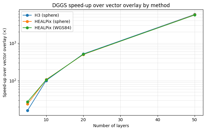

All three methods track each other closely and reach ~5000–5800× at 50 layers: the orders-of-magnitude advantage is a property of the DGGS approach, not of any one grid system.

Summary table¶

summary = load_json("results_comparison/comparison_summary.json")

import pandas as pd

method_rows = [
    {
        "method": name,
        "max_speedup": m["max_speedup"],
        "crossover_layers": round(m["crossover_layers"], 1),
    }
    for name, m in summary["methods"].items()
]
pd.DataFrame(method_rows)

Conclusions¶

Vector claim — validated. Across H3 and both HEALPix geometries, DGGS is orders of magnitude faster than vector overlay, and the gap grows with the number of layers.
Raster claim — validated. DGGS and raster classification are within a small constant factor, as the paper reports.
Extension finding. HEALPix matches H3 on performance, and the WGS84 ellipsoid correction is effectively free in time — but it materially changes cell assignment at mid- and high latitudes (see notebook 03).