pangeo_CMIP6_masked_and_weighted_average

Using masks and computing weighted average

This example is based from xarray example http://xarray.pydata.org/en/stable/examples/area_weighted_temperature.html

Import python packages

pip install nc-time-axis

Requirement already satisfied: nc-time-axis in /usr/share/miniconda/envs/repo/lib/python3.10/site-packages (1.4.1)
Requirement already satisfied: matplotlib in /usr/share/miniconda/envs/repo/lib/python3.10/site-packages (from nc-time-axis) (3.5.2)
Requirement already satisfied: cftime>=1.5 in /usr/share/miniconda/envs/repo/lib/python3.10/site-packages (from nc-time-axis) (1.6.0)
Requirement already satisfied: numpy in /usr/share/miniconda/envs/repo/lib/python3.10/site-packages (from nc-time-axis) (1.22.4)
Requirement already satisfied: pyparsing>=2.2.1 in /usr/share/miniconda/envs/repo/lib/python3.10/site-packages (from matplotlib->nc-time-axis) (3.0.9)
Requirement already satisfied: python-dateutil>=2.7 in /usr/share/miniconda/envs/repo/lib/python3.10/site-packages (from matplotlib->nc-time-axis) (2.8.2)
Requirement already satisfied: pillow>=6.2.0 in /usr/share/miniconda/envs/repo/lib/python3.10/site-packages (from matplotlib->nc-time-axis) (9.1.1)
Requirement already satisfied: fonttools>=4.22.0 in /usr/share/miniconda/envs/repo/lib/python3.10/site-packages (from matplotlib->nc-time-axis) (4.33.3)
Requirement already satisfied: packaging>=20.0 in /usr/share/miniconda/envs/repo/lib/python3.10/site-packages (from matplotlib->nc-time-axis) (21.3)
Requirement already satisfied: kiwisolver>=1.0.1 in /usr/share/miniconda/envs/repo/lib/python3.10/site-packages (from matplotlib->nc-time-axis) (1.4.2)
Requirement already satisfied: cycler>=0.10 in /usr/share/miniconda/envs/repo/lib/python3.10/site-packages (from matplotlib->nc-time-axis) (0.11.0)
Requirement already satisfied: six>=1.5 in /usr/share/miniconda/envs/repo/lib/python3.10/site-packages (from python-dateutil>=2.7->matplotlib->nc-time-axis) (1.16.0)
Note: you may need to restart the kernel to use updated packages.

import xarray as xr
xr.set_options(display_style='html')
import intake
import cftime
import matplotlib.pyplot as plt
import cartopy.crs as ccrs
import numpy as np
%matplotlib inline

cat_url = "https://storage.googleapis.com/cmip6/pangeo-cmip6.json"
col = intake.open_esm_datastore(cat_url)
col

pangeo-cmip6 catalog with 7686 dataset(s) from 514961 asset(s):

	unique
activity_id	18
institution_id	36
source_id	88
experiment_id	170
member_id	657
table_id	37
variable_id	700
grid_label	10
zstore	514961
dcpp_init_year	60
version	737

Search data

cat = col.search(source_id=['NorESM2-LM'], experiment_id=['historical'], table_id=['Amon'], variable_id=['tas'], member_id=['r1i1p1f1'])
cat.df

	activity_id	institution_id	source_id	experiment_id	member_id	table_id	variable_id	grid_label	zstore	dcpp_init_year	version
0	CMIP	NCC	NorESM2-LM	historical	r1i1p1f1	Amon	tas	gn	gs://cmip6/CMIP6/CMIP/NCC/NorESM2-LM/historica...	NaN	20190815

Create dictionary from the list of datasets we found

• This step may take several minutes so be patient!

dset_dict = cat.to_dataset_dict(zarr_kwargs={'use_cftime':True})

--> The keys in the returned dictionary of datasets are constructed as follows:
	'activity_id.institution_id.source_id.experiment_id.table_id.grid_label'

100.00% [1/1 00:00<00:00]

list(dset_dict.keys())

['CMIP.NCC.NorESM2-LM.historical.Amon.gn']

dset = dset_dict[list(dset_dict.keys())[0]]
dset

<xarray.Dataset>
Dimensions:    (lat: 96, bnds: 2, lon: 144, member_id: 1, time: 1980)
Coordinates:
    height     float64 ...
  * lat        (lat) float64 -90.0 -88.11 -86.21 -84.32 ... 86.21 88.11 90.0
    lat_bnds   (lat, bnds) float64 dask.array<chunksize=(96, 2), meta=np.ndarray>
  * lon        (lon) float64 0.0 2.5 5.0 7.5 10.0 ... 350.0 352.5 355.0 357.5
    lon_bnds   (lon, bnds) float64 dask.array<chunksize=(144, 2), meta=np.ndarray>
  * time       (time) object 1850-01-16 12:00:00 ... 2014-12-16 12:00:00
    time_bnds  (time, bnds) object dask.array<chunksize=(1980, 2), meta=np.ndarray>
  * member_id  (member_id) <U8 'r1i1p1f1'
Dimensions without coordinates: bnds
Data variables:
    tas        (member_id, time, lat, lon) float32 dask.array<chunksize=(1, 990, 96, 144), meta=np.ndarray>
Attributes: (12/54)
    Conventions:               CF-1.7 CMIP-6.2
    activity_id:               CMIP
    branch_method:             Hybrid-restart from year 1600-01-01 of piControl
    branch_time:               0.0
    branch_time_in_child:      0.0
    branch_time_in_parent:     430335.0
    ...                        ...
    variable_id:               tas
    variant_label:             r1i1p1f1
    netcdf_tracking_ids:       hdl:21.14100/2486cf87-033c-4848-ab3e-e828c3b7c...
    version_id:                v20190815
    intake_esm_varname:        ['tas']
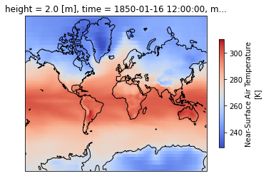
    intake_esm_dataset_key:    CMIP.NCC.NorESM2-LM.historical.Amon.gn

xarray.Dataset

• Dimensions:
  • lat: 96
  • bnds: 2
  • lon: 144
  • member_id: 1
  • time: 1980
• Coordinates: (8)
  • height
    ()
    float64
    ...

    axis :

    Z

    long_name :

    height

    positive :

    up

    standard_name :

    height

    units :

    m

    array(2.)

  • lat
    (lat)
    float64
    -90.0 -88.11 -86.21 ... 88.11 90.0

    axis :

    Y

    bounds :

    lat_bnds

    long_name :

    Latitude

    standard_name :

    latitude

    units :

    degrees_north

    array([-90.      , -88.105263, -86.210526, -84.315789, -82.421053, -80.526316,
           -78.631579, -76.736842, -74.842105, -72.947368, -71.052632, -69.157895,
           -67.263158, -65.368421, -63.473684, -61.578947, -59.684211, -57.789474,
           -55.894737, -54.      , -52.105263, -50.210526, -48.315789, -46.421053,
           -44.526316, -42.631579, -40.736842, -38.842105, -36.947368, -35.052632,
           -33.157895, -31.263158, -29.368421, -27.473684, -25.578947, -23.684211,
           -21.789474, -19.894737, -18.      , -16.105263, -14.210526, -12.315789,
           -10.421053,  -8.526316,  -6.631579,  -4.736842,  -2.842105,  -0.947368,
             0.947368,   2.842105,   4.736842,   6.631579,   8.526316,  10.421053,
            12.315789,  14.210526,  16.105263,  18.      ,  19.894737,  21.789474,
            23.684211,  25.578947,  27.473684,  29.368421,  31.263158,  33.157895,
            35.052632,  36.947368,  38.842105,  40.736842,  42.631579,  44.526316,
            46.421053,  48.315789,  50.210526,  52.105263,  54.      ,  55.894737,
            57.789474,  59.684211,  61.578947,  63.473684,  65.368421,  67.263158,
            69.157895,  71.052632,  72.947368,  74.842105,  76.736842,  78.631579,
            80.526316,  82.421053,  84.315789,  86.210526,  88.105263,  90.      ])

  • lat_bnds
    (lat, bnds)
    float64
    dask.array<chunksize=(96, 2), meta=np.ndarray>

    Array Chunk Bytes 1.50 kiB 1.50 kiB Shape (96, 2) (96, 2) Count 2 Tasks 1 Chunks Type float64 numpy.ndarray

  • lon
    (lon)
    float64
    0.0 2.5 5.0 ... 352.5 355.0 357.5

    axis :

    X

    bounds :

    lon_bnds

    long_name :

    Longitude

    standard_name :

    longitude

    units :

    degrees_east

    array([  0. ,   2.5,   5. ,   7.5,  10. ,  12.5,  15. ,  17.5,  20. ,  22.5,
            25. ,  27.5,  30. ,  32.5,  35. ,  37.5,  40. ,  42.5,  45. ,  47.5,
            50. ,  52.5,  55. ,  57.5,  60. ,  62.5,  65. ,  67.5,  70. ,  72.5,
            75. ,  77.5,  80. ,  82.5,  85. ,  87.5,  90. ,  92.5,  95. ,  97.5,
           100. , 102.5, 105. , 107.5, 110. , 112.5, 115. , 117.5, 120. , 122.5,
           125. , 127.5, 130. , 132.5, 135. , 137.5, 140. , 142.5, 145. , 147.5,
           150. , 152.5, 155. , 157.5, 160. , 162.5, 165. , 167.5, 170. , 172.5,
           175. , 177.5, 180. , 182.5, 185. , 187.5, 190. , 192.5, 195. , 197.5,
           200. , 202.5, 205. , 207.5, 210. , 212.5, 215. , 217.5, 220. , 222.5,
           225. , 227.5, 230. , 232.5, 235. , 237.5, 240. , 242.5, 245. , 247.5,
           250. , 252.5, 255. , 257.5, 260. , 262.5, 265. , 267.5, 270. , 272.5,
           275. , 277.5, 280. , 282.5, 285. , 287.5, 290. , 292.5, 295. , 297.5,
           300. , 302.5, 305. , 307.5, 310. , 312.5, 315. , 317.5, 320. , 322.5,
           325. , 327.5, 330. , 332.5, 335. , 337.5, 340. , 342.5, 345. , 347.5,
           350. , 352.5, 355. , 357.5])

  • lon_bnds
    (lon, bnds)
    float64
    dask.array<chunksize=(144, 2), meta=np.ndarray>

    Array Chunk Bytes 2.25 kiB 2.25 kiB Shape (144, 2) (144, 2) Count 2 Tasks 1 Chunks Type float64 numpy.ndarray

  • time
    (time)
    object
    1850-01-16 12:00:00 ... 2014-12-...

    axis :

    T

    bounds :

    time_bnds

    long_name :

    time

    standard_name :

    time

    array([cftime.DatetimeNoLeap(1850, 1, 16, 12, 0, 0, 0, has_year_zero=True),
           cftime.DatetimeNoLeap(1850, 2, 15, 0, 0, 0, 0, has_year_zero=True),
           cftime.DatetimeNoLeap(1850, 3, 16, 12, 0, 0, 0, has_year_zero=True),
           ...,
           cftime.DatetimeNoLeap(2014, 10, 16, 12, 0, 0, 0, has_year_zero=True),
           cftime.DatetimeNoLeap(2014, 11, 16, 0, 0, 0, 0, has_year_zero=True),
           cftime.DatetimeNoLeap(2014, 12, 16, 12, 0, 0, 0, has_year_zero=True)],
          dtype=object)

  • time_bnds
    (time, bnds)
    object
    dask.array<chunksize=(1980, 2), meta=np.ndarray>

    Array Chunk Bytes 30.94 kiB 30.94 kiB Shape (1980, 2) (1980, 2) Count 2 Tasks 1 Chunks Type object numpy.ndarray

  • member_id
    (member_id)
    <U8
    'r1i1p1f1'

    array(['r1i1p1f1'], dtype='<U8')

• Data variables: (1)
  • tas
    (member_id, time, lat, lon)
    float32
    dask.array<chunksize=(1, 990, 96, 144), meta=np.ndarray>

    cell_measures :

    area: areacella

    cell_methods :

    area: time: mean

    comment :

    near-surface (usually, 2 meter) air temperature

    history :

    2019-08-15T12:42:20Z altered by CMOR: Treated scalar dimension: 'height'. 2019-08-15T12:42:21Z altered by CMOR: Converted type from 'd' to 'f'.

    long_name :

    Near-Surface Air Temperature

    original_name :

    TREFHT

    standard_name :

    air_temperature

    units :

    K

    Array Chunk Bytes 104.41 MiB 52.21 MiB Shape (1, 1980, 96, 144) (1, 990, 96, 144) Count 5 Tasks 2 Chunks Type float32 numpy.ndarray

• Attributes: (54)

  Conventions :

  CF-1.7 CMIP-6.2

  activity_id :

  CMIP

  branch_method :

  Hybrid-restart from year 1600-01-01 of piControl

  branch_time :

  0.0

  branch_time_in_child :

  0.0

  branch_time_in_parent :

  430335.0

  cmor_version :

  3.5.0

  contact :

  Please send any requests or bug reports to noresm-ncc@met.no.

  creation_date :

  2019-08-15T12:42:21Z

  data_specs_version :

  01.00.31

  experiment :

  all-forcing simulation of the recent past

  experiment_id :

  historical

  external_variables :

  areacella

  forcing_index :

  1

  frequency :

  mon

  further_info_url :

  https://furtherinfo.es-doc.org/CMIP6.NCC.NorESM2-LM.historical.none.r1i1p1f1

  grid :

  finite-volume grid with 1.9x2.5 degree lat/lon resolution

  grid_label :

  gn

  history :

  2019-08-15T12:42:21Z ; CMOR rewrote data to be consistent with CMIP6, CF-1.7 CMIP-6.2 and CF standards.

  initialization_index :

  1

  institution :

  NorESM Climate modeling Consortium consisting of CICERO (Center for International Climate and Environmental Research, Oslo 0349), MET-Norway (Norwegian Meteorological Institute, Oslo 0313), NERSC (Nansen Environmental and Remote Sensing Center, Bergen 5006), NILU (Norwegian Institute for Air Research, Kjeller 2027), UiB (University of Bergen, Bergen 5007), UiO (University of Oslo, Oslo 0313) and UNI (Uni Research, Bergen 5008), Norway. Mailing address: NCC, c/o MET-Norway, Henrik Mohns plass 1, Oslo 0313, Norway

  institution_id :

  NCC

  license :

  CMIP6 model data produced by NCC is licensed under a Creative Commons Attribution ShareAlike 4.0 International License (https://creativecommons.org/licenses). Consult https://pcmdi.llnl.gov/CMIP6/TermsOfUse for terms of use governing CMIP6 output, including citation requirements and proper acknowledgment. Further information about this data, including some limitations, can be found via the further_info_url (recorded as a global attribute in this file) and at https:///pcmdi.llnl.gov/. The data producers and data providers make no warranty, either express or implied, including, but not limited to, warranties of merchantability and fitness for a particular purpose. All liabilities arising from the supply of the information (including any liability arising in negligence) are excluded to the fullest extent permitted by law.

  mip_era :

  CMIP6

  model_id :

  NorESM2-LM

  nominal_resolution :

  250 km

  parent_activity_id :

  CMIP

  parent_experiment_id :

  piControl

  parent_mip_era :

  CMIP6

  parent_source_id :

  NorESM2-LM

  parent_sub_experiment_id :

  none

  parent_time_units :

  days since 0421-01-01

  parent_variant_label :

  r1i1p1f1

  physics_index :

  1

  product :

  model-output

  realization_index :

  1

  realm :

  atmos

  run_variant :

  N/A

  source :

  NorESM2-LM (2017): aerosol: OsloAero atmos: CAM-OSLO (2 degree resolution; 144 x 96; 32 levels; top level 3 mb) atmosChem: OsloChemSimp land: CLM landIce: CISM ocean: MICOM (1 degree resolution; 360 x 384; 70 levels; top grid cell minimum 0-2.5 m [native model uses hybrid density and generic upper-layer coordinate interpolated to z-level for contributed data]) ocnBgchem: HAMOCC seaIce: CICE

  source_id :

  NorESM2-LM

  source_type :

  AOGCM

  status :

  2020-04-30;created; by gcs.cmip6.ldeo@gmail.com

  sub_experiment :

  none

  sub_experiment_id :

  none

  table_id :

  Amon

  table_info :

  Creation Date:(24 July 2019) MD5:08e314340b9dd440c36c1b8e484514f4

  title :

  NorESM2-LM output prepared for CMIP6

  tracking_id :

  hdl:21.14100/2486cf87-033c-4848-ab3e-e828c3b7c759 hdl:21.14100/8d2ec216-30d3-4f90-8664-7cf75e29780b hdl:21.14100/9f798305-d0cf-4eac-89b0-b13dc25574ca hdl:21.14100/e0da9277-4784-446b-b3b5-ba33bb18cc3a hdl:21.14100/ca48487c-955a-4b15-9582-5ce55ce39c73 hdl:21.14100/fc7602aa-fd09-49d8-94c6-e619622c211b hdl:21.14100/cd51a9c2-0a94-45b2-8d9b-59bcb3467214 hdl:21.14100/9b7ad334-1217-4229-98e8-b5a9287c0e5e hdl:21.14100/043ca527-40c7-451f-990b-ccc94720f612 hdl:21.14100/a9613498-ea0d-4be4-97e8-77661872798d hdl:21.14100/52699832-d86c-491b-a0a4-2f27d9ee4d69 hdl:21.14100/358c4a18-33b2-4c44-bd30-f6125a4df63c hdl:21.14100/77254eaf-90ca-44e7-9a3c-763a840e188f hdl:21.14100/62aed49c-6ca5-4027-80fe-4ddd99af575a hdl:21.14100/83ffe172-769b-42b1-b979-b92d768f60fd hdl:21.14100/91a8c4e2-d33b-4b87-a978-0247d8112ef3 hdl:21.14100/e8fb384f-d5a7-41e1-bf12-b8de3e2ffb80

  variable_id :

  tas

  variant_label :

  r1i1p1f1

  netcdf_tracking_ids :

  hdl:21.14100/2486cf87-033c-4848-ab3e-e828c3b7c759 hdl:21.14100/8d2ec216-30d3-4f90-8664-7cf75e29780b hdl:21.14100/9f798305-d0cf-4eac-89b0-b13dc25574ca hdl:21.14100/e0da9277-4784-446b-b3b5-ba33bb18cc3a hdl:21.14100/ca48487c-955a-4b15-9582-5ce55ce39c73 hdl:21.14100/fc7602aa-fd09-49d8-94c6-e619622c211b hdl:21.14100/cd51a9c2-0a94-45b2-8d9b-59bcb3467214 hdl:21.14100/9b7ad334-1217-4229-98e8-b5a9287c0e5e hdl:21.14100/043ca527-40c7-451f-990b-ccc94720f612 hdl:21.14100/a9613498-ea0d-4be4-97e8-77661872798d hdl:21.14100/52699832-d86c-491b-a0a4-2f27d9ee4d69 hdl:21.14100/358c4a18-33b2-4c44-bd30-f6125a4df63c hdl:21.14100/77254eaf-90ca-44e7-9a3c-763a840e188f hdl:21.14100/62aed49c-6ca5-4027-80fe-4ddd99af575a hdl:21.14100/83ffe172-769b-42b1-b979-b92d768f60fd hdl:21.14100/91a8c4e2-d33b-4b87-a978-0247d8112ef3 hdl:21.14100/e8fb384f-d5a7-41e1-bf12-b8de3e2ffb80

  version_id :

  v20190815

  intake_esm_varname :

  ['tas']

  intake_esm_dataset_key :

  CMIP.NCC.NorESM2-LM.historical.Amon.gn

Plot the first timestep

projection = ccrs.Mercator(central_longitude=-10)

f, ax = plt.subplots(subplot_kw=dict(projection=projection))

dset['tas'].isel(time=0).plot(transform=ccrs.PlateCarree(), cbar_kwargs=dict(shrink=0.7), cmap='coolwarm')
ax.coastlines()

<cartopy.mpl.feature_artist.FeatureArtist at 0x7f1212118670>

Compute weighted mean

1. Creating weights: for a rectangular grid the cosine of the latitude is proportional to the grid cell area.
2. Compute weighted mean values

def computeWeightedMean(ds):
    # Compute weights based on the xarray you pass
    weights = np.cos(np.deg2rad(ds.lat))
    weights.name = "weights"
    # Compute weighted mean
    air_weighted = ds.weighted(weights)
    weighted_mean = air_weighted.mean(("lon", "lat"))
    return weighted_mean

Compute weighted average over the entire globe

weighted_mean = computeWeightedMean(dset)

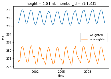
Comparison with unweighted mean

• We select a time range
• Note how the weighted mean temperature is higher than the unweighted.

weighted_mean['tas'].sel(time=slice('2000-01-01', '2010-01-01')).plot(label="weighted")
dset['tas'].sel(time=slice('2000-01-01', '2010-01-01')).mean(("lon", "lat")).plot(label="unweighted")

plt.legend()

<matplotlib.legend.Legend at 0x7f12138a66b0>

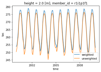
Compute Weigted arctic average

Let’s try to also take only the data above 60$^\circ$

weighted_mean = computeWeightedMean(dset.where(dset['lat']>60.))

weighted_mean['tas'].sel(time=slice('2000-01-01', '2010-01-01')).plot(label="weighted")
dset['tas'].where(dset['lat']>60.).sel(time=slice('2000-01-01', '2010-01-01')).mean(("lon", "lat")).plot(label="unweighted")

plt.legend()

<matplotlib.legend.Legend at 0x7f1211b59480>

This site is open source. Improve this page.